5. Multiprocessor scheduling services

5.1 Global multiprocessor scheduling

5.2 Cache interference analysis

Cache interference in Cheddar is based on the concepts of Cache Related Preemption Delay (CRPD). The bounds on the CRPD are computed by using :
- Useful Cache Block [LEE 98]
- Evicting Cache Block[BUS 95]
The following process is required to run the CRPD analyses implemented in Cheddar.

1. Control Flow Graph (CFG) computation.

Cheddar provides supports for modeling the CFG of a task. An external tool is used to parse the object file of a task and then to compute and generate the CFG in a Cheddar-compatible format. Examples of the CFGs computed for tasks in the Malardalen benchmark are available on the Cheddar svn repository at this link.
2. Import/create a Cheddar-ADL system model and import its CFGs

The users can import an existing system model with several tasks in Cheddar or choose to create a new model. After that, the CFGs of these tasks can imported by Cheddar :
```
Menu --> Tools --> Cache --> Import Control Flow Graph
```
- If the users import a Cheddar-ADL system model, the CFGs must be located in the same folder as the xml file.
- If the users create a new system model, the CFGs must be located in the same folder with the Chedder executable file.
- The attribute "cfg_name" is used to associate a CFG to a task. The xml file contains the CFG must has the same name as Cheddar automatically search for the CFGs to be imported.
The current GUI of Cheddar does not provide an interactive way to work (add/modify/delete) with CFGs. The features are to be implemented in the next version.
3. UCBs and ECBs computation

The sets of UCBs and ECBs of a program are computed by Cheddar from its CFG.

The sets of UCBs and ECBs can also be computed by external tools and put directly in Cheddar without passing by this step. In order to do this, the users need to modify the xml file of a Cheddar-ADL system model with the information about the UCBs and ECBs of tasks.

After this step, the following analyses are available in Cheddar

4.1 CRPD-Aware WCRT analysis

In order to perform CRPD-Aware WCRT analysis in Cheddar, the following steps are required:
- The set of UCBs and ECBs of all tasks must be computed (Step 3).
- Menu --> Tools --> Scheduling --> Feasibility Test Options
- The following tests are available in Cheddar:
  - ECB-Only [LEE 98]
  - ECB-Union Multi-set [ALT 12]
  - UCB-Union Multi-set [ALT 12]
  - Combined Multi-set [ALT 12]
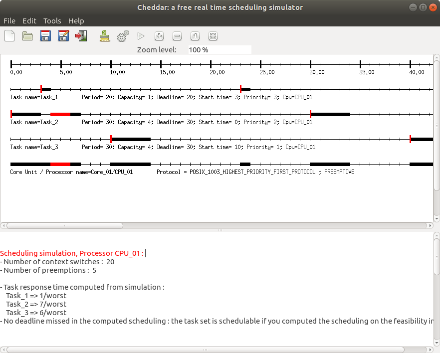
4.2 CRPD-Aware Scheduling Simulation [TRA 16a]

In order to perform CRPD-aware scheduling simulation in Cheddar, the following steps are required.
- The set of UCBs and ECBs of all tasks must be computed (Step 3).
- Check the CRPD check box in Tools --> Scheduling --> Scheduling Options
- Run the simulation. The CRPD added to the capacities of tasks are represented by the red blocks (as shown in the image below)
4.3 CRPD-Aware Prority Assignment [TRA 16b]

Our implementation of the CRPD-aware priority assignment is based on Audsley's Optimal Priority Assignment (OPA) algorithm. We extended this algorithm in order to take into account the CRPD. In order to perform CRPD-aware prority assignment in Cheddar, the following steps are required.
- The set of UCBs and ECBs of all tasks must be computed (Step 3).
- Tools --> Scheduling --> Scheduling Options --> Tasks Priority Assignment
- The following CRPD priority assignment algorithms, which are detailed in the referenced article, are available in Cheddar:
  - CRPD OPA-PT
  - CRPD OPA-PT Simplified
  - CRPD OPA-PT Tree

5.3 Memory interference analysis

5.4 Network-On-Chip interference analysis

5.5 Partitionning algorithms

Multiprocessor system is good for heavy computing demands. It is sometimes the only way to provide sufficient processing power to meet critical real-time deadlines. In general multiprocessor systems are also more reliable than uni-processor systems. Scheduling of multiprocessor systems is proven to be a NP-hard (Non-deterministic Polynomial-time) problem [LEU 82]. The complexity class NP is the set of decision problems that can be solved by a non-deterministic machine in polynomial time. The complexity theory is part of the theory of computation dealing with the resources required during computation to solve a given problem. The most common resources are time (how many steps does it take to solve a problem) and space (how much memory does it take to solve a problem). Other resources can also be considered, such as how many parallel processors are needed to solve a problem in parallel. There are many scheduling heuristics to solve this. Rate-monotonic scheduling is good for numerous reasons: Rate-monotonic algorithm is optimal for fixed priority assignment of periodic tasks on a processor so it�s easy to design predictable real-time system. Also it is easy to implement and it takes minimal scheduling overhead.

Cheddar has four algorithms: RMNF, RMFF, RMBF, RMST and RMGT. Each of these are off-line schemes, so the entire task set must be known before starting task assignment. Bounds for functions are calculated using .

Rate-Monotonic-Next-Fit [SON 93]

Upper bound for this algorithm is 2.67. Tasks are sorted in non-decreasing order of periods. Then tasks are placed on processors, according to the IP Condition (Increasing Period). The first task is placed on the first processor. Then the second task is placed on the first processor, if it meets the IP Condition. Otherwise it is placed on a new processor. This continues until all tasks are scheduled.

Rate-Monotonic-First-Fit [SON 93]

The upper bound for this algorithm is 2.33 [SON 93] (original study by Liu and Dhall had a wrong bound of 2.23). Tasks are sorted in non-decreasing order of periods. The IP Condition is used to verify teh schedulability of tasks on processors. The first task is placed on the first processor. Then the second task is placed on the first processor, if it meets the IP Condition. Otherwise it is placed on a new processor. The third task is tried to be placed on the first processor according to the IP Condition. If it does not meet the condition, the task is tried to be placed on the second processor. Otherwise a new processor is selected for the third task�

Rate-Monotonic-Best-Fit [SON 93]

The upper bound for this algorithm is 2.33. Tasks are sorted in non-decreasing order of periods. The first task is placed on the first processor. For the second task, the function checks all processors, whether they meet the IP Condition. For processors that satisfy the condition, the algorithm checks the number kj of tasks already assigned to each processor j, and computes Uj, the total utilization of the kj tasks. And the task is assigned to the processor that has the smallest value. If the condition is not met, a new processor is selected for the task.

Rate-Monotonic Small-Tasks [BUR 94]

The upper bound for RMST is , a = max Ui, i = 1,�,K and U is utilization of all tasks. Tasks are sorted in increasing Si. Si = log2(Ti). The main idea of RMST is to minimize the value of b for each processor. � = max Si � min Si, 1= i =K.

Rate-Monotonic General-Tasks [BUR 94]

The upper bound for RMGT is 1.75. RMGT uses the RMST algorithm for task s = 1/3 and First-Fit heuristics for the rest of the tasks.

Example of use :

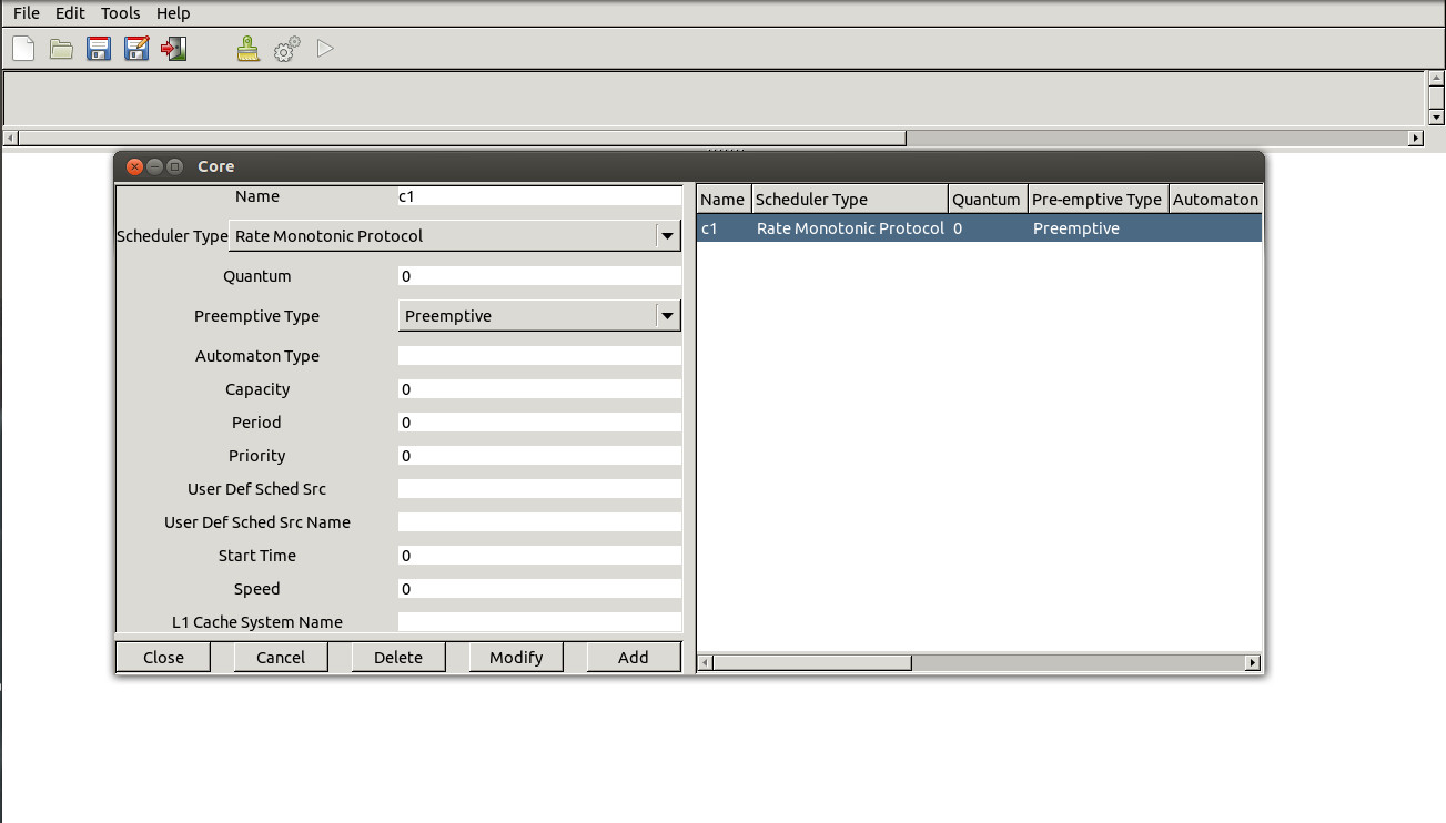
First, Define cores for processors. They have to be of Rate Monotonic type.
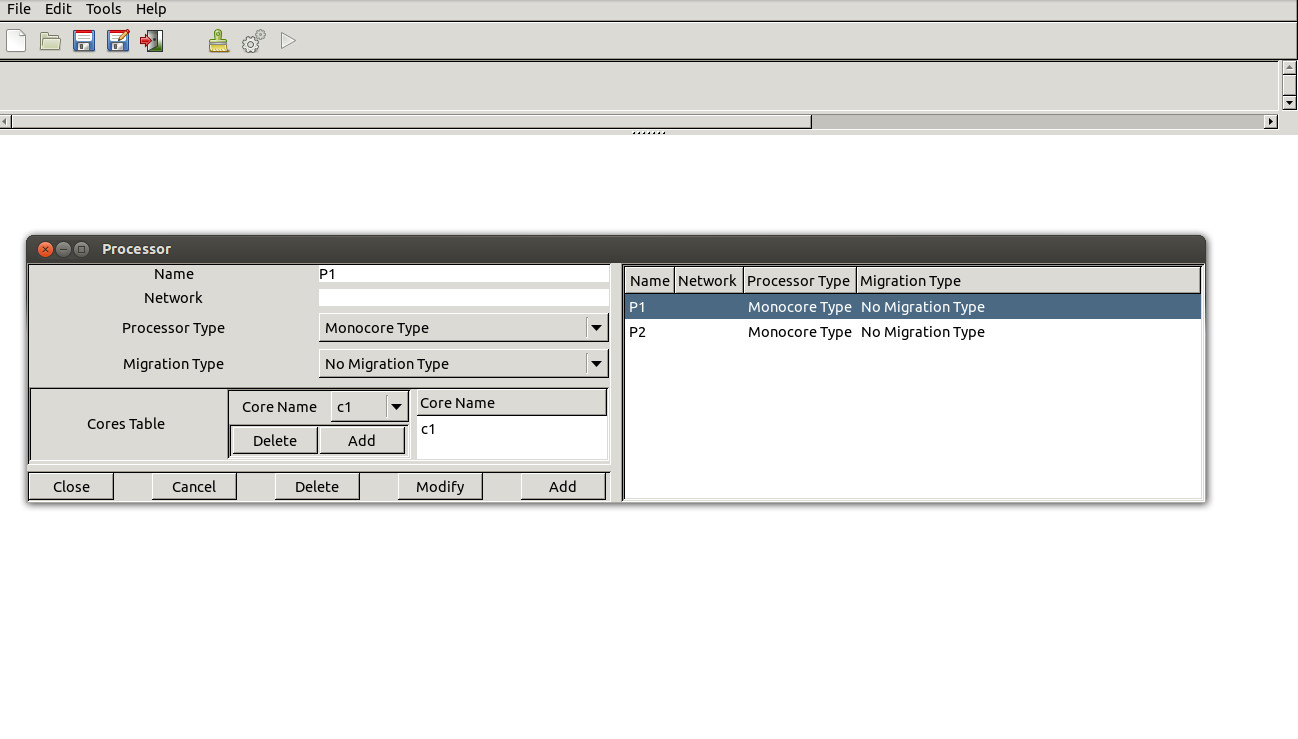
Second, Define processors for tasks.
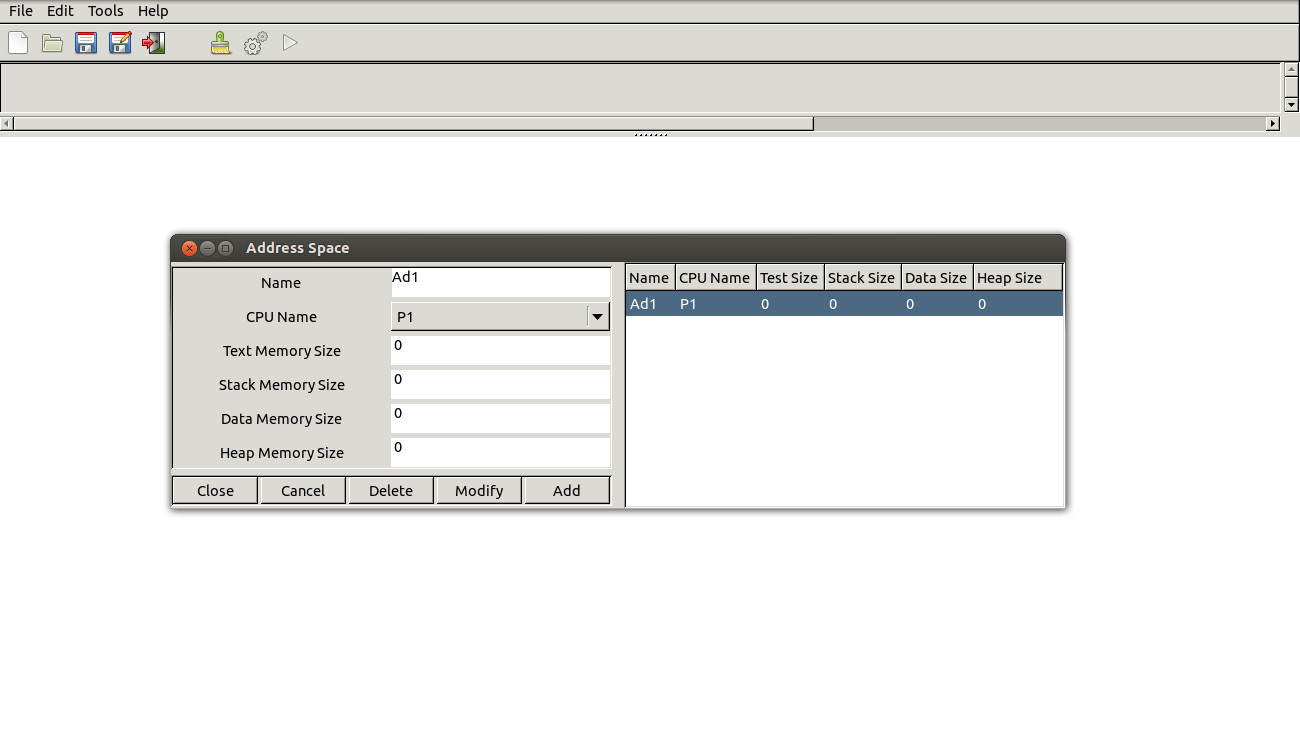
Third, Define Address space used by tasks.
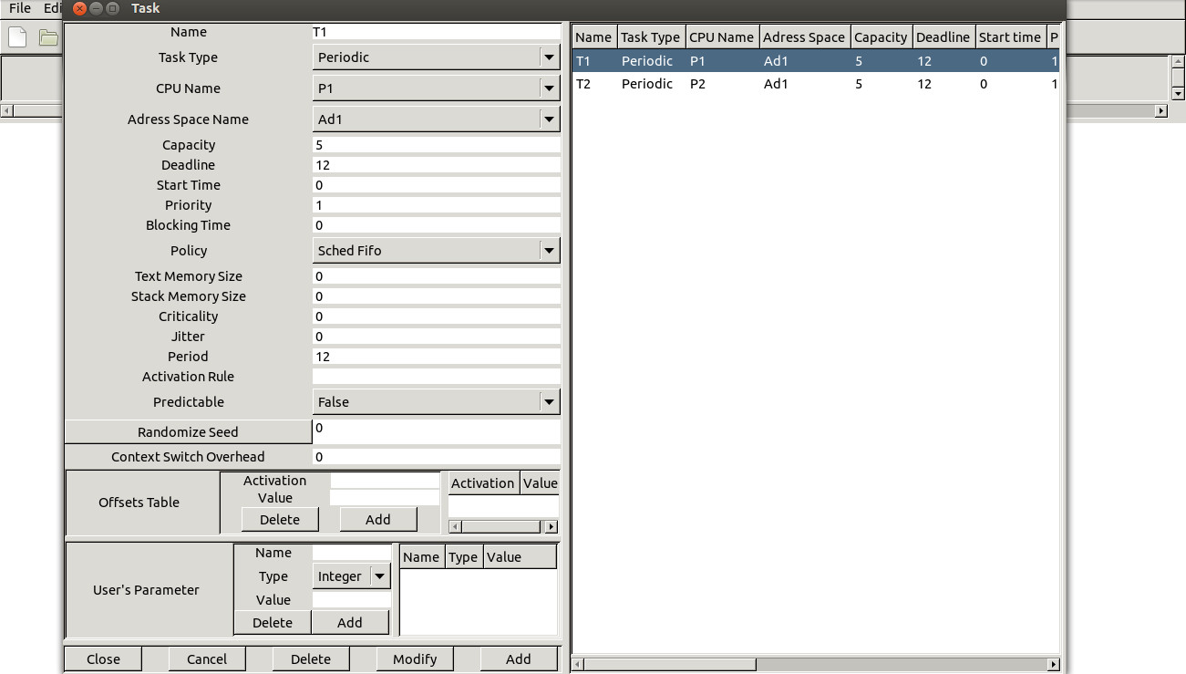
Then, Define tasks (host tasks on any processor and address space)
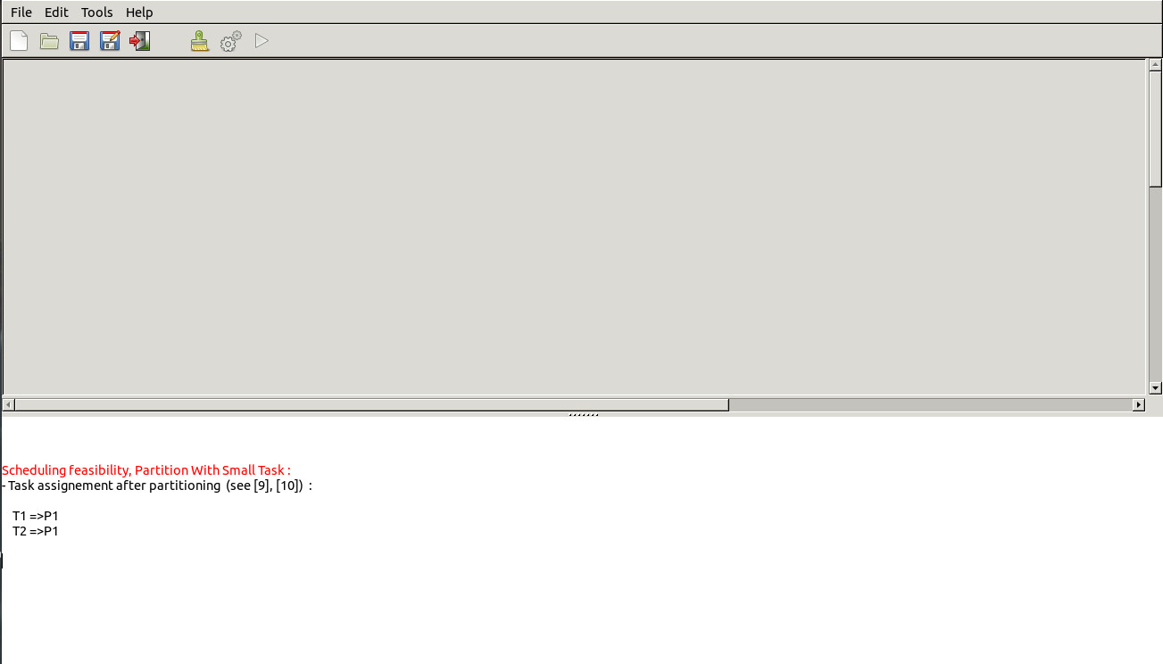
Finally, compute partitioning, with the submenu "Tool/Scheduling/Partition/With Small Task". :