1. Basic features: scheduling simulation and feasibility tests for independent tasks

In this chapter, you find a description of the most important scheduling and feasibility services provided by Cheddar in the case of independent tasks.

1.1 First step: a simple scheduling simulation

This section shows you how to call the simpliest features of Cheddar.

Cheddar provides tools to check temporal constraints of real time tasks. These tools are based on classical results from real time scheduling theory. Before calling such tools, you have to define a system which is mainly composed of several processors and tasks.

To define a processor, you should first define one or multiple cores. For that choose the "Edit/Hardware/Core" submenu. The window below is then displayed:

Figure 1.1 Adding a core

A core is defined by the following fields (see Figure 1.1):

The name of the core. A core name can be any combination of literal characters including underscore. Space is forbidden. Each core must have a unique name.
The scheduler hosted by the core. Basically, you can choose from a various set of schedulers such as (to get a detailed description on these schedulers, see section Other Available schedulers and task arrival patterns):
- "Earliest Deadline First" (or EDF). Tasks can be periodic or not and are scheduled according to their deadline.
- "Least Laxity First" (or LLF). Tasks can be periodic or not and are scheduled according to their laxity. The laxity is computed by : L_i = D_i - C'_i in which L_i is the laxity of the task, D_i is the deadline, and C'_i is the remaining capacity.
- "Least Runtime Laxity First" (a second interpretation of LLF). Tasks can be periodic or not and are scheduled according to their laxity. The laxity is computed by : L_i = D_i - (C'_i + t_i) in which L_i is the laxity of the task, D_i is the deadline, C'_i is the remaining capacity, and t_i is the time passed since the release time of the task.
- "Rate Monotonic" (or RM, or RMA, or RMS). Tasks have to be periodic, and deadline must be equal to period. Tasks are scheduled according to their period. You have to be aware that the value of the priority field of the tasks is ignored here.
- "Deadline Monotonic" (or DM). Tasks have to be periodic and are scheduled according to their deadline. You have to be aware that the value of the priority field of the tasks is ignored here.
- "Posix 1003 Highest Priority First". Tasks can be periodic or not. Tasks are scheduled according to the priority and the policy of the tasks. (Rate Monotonic and Deadline Monotonic use the same scheduler engine except that priorities are automatically computed from task period or deadline). POSIX 1003.1b scheduler supports SCHED_RR, SCHED_FIFO and SCHED_OTHERS queueing policies. SCHED_OTHERS is a time sharing policy. SCHED_RR and SCHED_FIFO tasks must have priorities ranging between 255 and 1. Priority level 0 is reserved for SCHED_OTHERS tasks. The highiest priority level is 255.
- "Time sharing based on wait time" (which is a Linux-like scheduler) and "Time sharing based on cpu usage". These two schedulers provide a way to share the processor as on a time sharing operatong system. With the first scheduler, the more a ready task waits for the processor and the more its priority increases. With the second scheduler, the more a ready task uses the processor and the more its priority decreases.
- "Round robin" (with quantum). The processor is regulary shared between all the tasks. A quantum (which is a bound on the time a task keeps the processor) can be given.
- "Maximum Urgency First based on laxity" and "Maximum Urgency First based on deadline". Such schedulers are based on an hybrid priority assignment : a task priority is made of a fixed part and a dynamic part (see ).
- "D-Over". This scheduler is an EDF like but which is work fine when the processor is over-loaded. When the processor is over-loaded, D-Over is always able to predict which tasks will miss its deadline (in contrary to EDF).
- User-defined schedulers ("Pipeline user-defined scheduler", "Automata user-defined scheduler" or "Compiled user-defined scheduler"). These schedulers allow users to define their own scheduler into Cheddar (see section User Defined Scheduler for details).
If the scheduler is preemptive or not. By default, the scheduler is set to be preemptive.
The quantum value associated with the scheduler. This information is useful if a scheduler has to manage several tasks with the same dynamic or static priority : in this case, the simulator has to choose how to share the processor between these tasks. The quantum is a bound on the delay a task can hold the processor (if the quantum is equal to zero, there is no bound on the processor holding time). At the time we're speaking, the quantum value can be used with the POSIX 1003.1b scheduler (only with SCHED_RR tasks) and the round robin scheduler. With POSIX 1003.1b, two SCHED_RR tasks with the same priority level should share the processor with a POSIX round-robin policy. In this case, the quantum value is the time slot of this round-robin scheduler. Finally, the quantum value could also be used for user-defined scheduler (see User Defined Scheduler for details).
Automaton name: user-defined scheduler can be expressed as an automaton. In this case, the this attribute stores the name of the automaton for the given core.
Capacity, Period, and Priority: These attributes are used to perform scheduling analysis with a polling server, for more information see Hierachical Scheduler
The User Defined Scheduler Source File Name is the name of a file which contains the source code of a user-defined scheduler (see section User Defined Scheduler for details).
Start time: time of the first release of the task
Speed. This attribute is the speed of the core. Default value is 1 and only positive non null values are accepted for this attribute. When the value of this attribute is equal to n, it means that task are executed n times quicker.
L1 Cache system name: This attribute indicate which cache is used to the core unit.

Warning: with Cheddar, to add a core (or any object), you have to push the Add button before pushing the Close button. That allows you to define several objects quickly without closing the window (you should then push Add for each defined object).

Then you can define a processor. For that choose the "Edit/Entities/Hardware/Processor" submenu. The window below is then displayed:

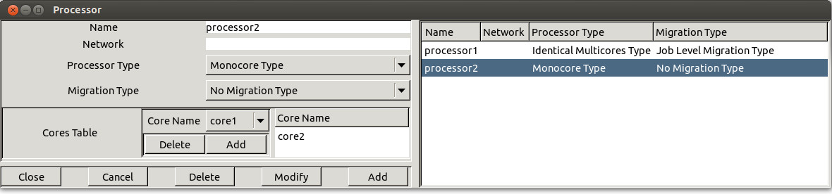
Figure 1.2 Adding a processor

A processor is defined by the following fields (see Figure 1.2) :

The name of the processor. A processor name can be any combination of literal characters including underscore. Space is forbidden. Each processor must have a unique name.
At the time we're speaking, the network field is not used (planned to be used in order to simulate message scheduling).
Processor type 4 kinds of processor exists in Cheddar:
- Monocore type. It contains only one core and can run only one task at a time.
- Identical multicores type. The processor contains several cores that are identical, i.e. have the same scheduling protocol (but with potentionnaly different parameters). All core of such processor have the same speed.
- Uniform multicores type. The processor contains cores that have different speeds. However speeds have proportional values. All cores of the same processor have to run the same scheduling protocol.
- Unrelated multicores type. The processor contains cores with differents speeds. Speeds have unrelated values. Again, all cores of the same processor have to run the same scheduling protocol.
Migration type . This attributes specifies how the tasks are allowed to move from one core to another.
- No migration type. Task cannot move from one core to another. This is typically the case of Multicore ARINC 653 architectures, or also of architectures with the concepts of core affinity (i.e. POSIX standard).
- Job level migration type. A task running on a core can move to another core only when its current job is completed. Running the smae job on two different cores is not allowed.
- Time unit migration type. A task can migrate at any core at any time.
Cores table which contain the list of cores initially defined. The user should select one core in the monocore processor case, and almost one core in other case.

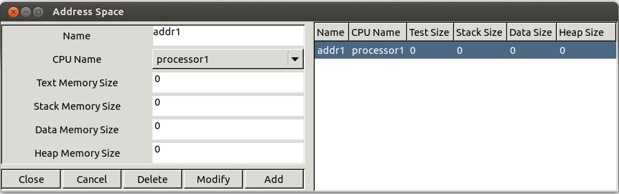
Figure 1.3 Adding an address space

The next step in order to run a simulation, is to define an address space. Choose the "Edit/Entities/Software/Address space" submenu. An address space models a piece of memory which contain tasks, buffers or shared resources. The Figure 1.3 shows the widget used to define such a feature. At the time we are speaking, the information you have to provide is:

A name. An address space name can be any combination of literal characters including underscore. Space is forbidden. Each address space name has to be unique.
A processor name. This is the processor which hosts the address space.
Some fields related to the size of the address space memory: the text memory size, the heap memory size, the stack memory size and the data memory size. The fields related to memory size will be used in the next Cheddar's release in order to perform a global memory analysis.

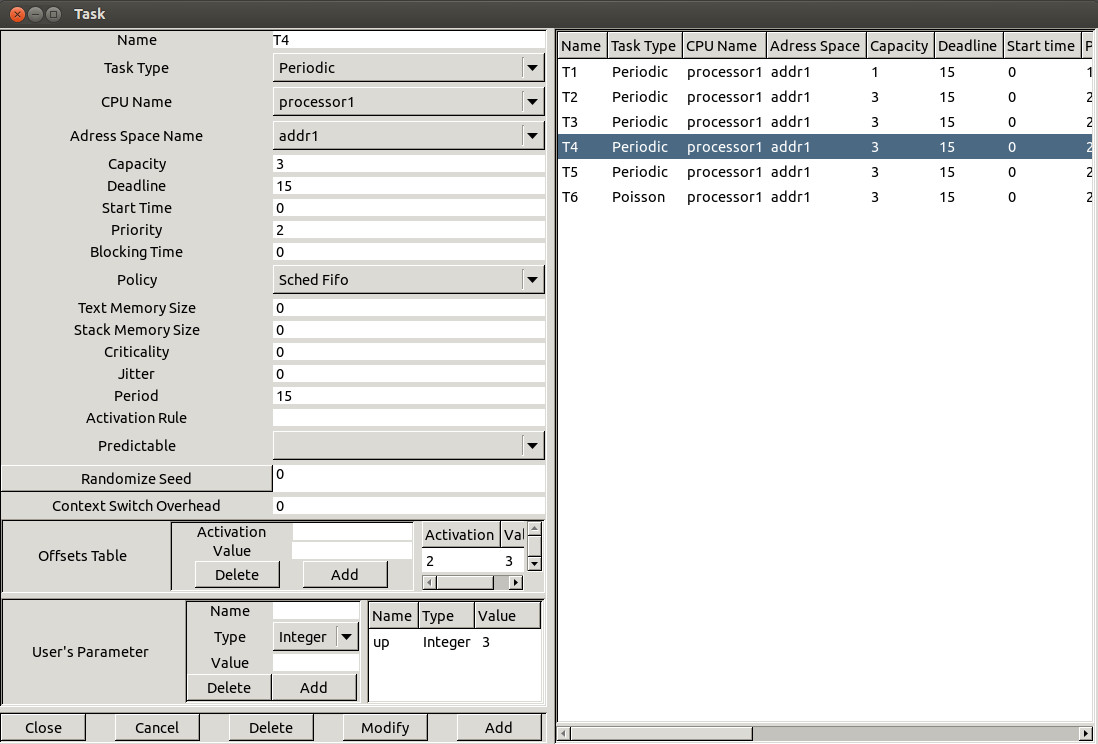
Figure 1.4 Adding a task

Let see now, how to define a task, the last feature required to perform the most simpliest performance analysis. Choose the "Edit/Entities/Software/Task" submenu. The window of Figure 1.4 is then displayed. This window is composed of 3 sub-parts : the "main part", the "offset part" and the "user's defined parameters part". The main part contains the following informations :

At least, a task is defined by a name (the task name should be unique), a capacity (bound on its execution time) and a place to run it (a processor name and an address space name). The other parameters are optional but can be required for a particular scheduler
A type of task . It describes the way the task is activated. An aperiodic task is only activated once. A periodic task is activated many times and the delay between two activations is a fixed one. A poisson process task is activated many times and the delay between two activations is a random delay : the random law used to generated these delays is an exponential one (poisson process). a sporadic task is a task which is activated many times with a minimal delay between two succesive activations. If the task type is "user-defined", the task activation law is defined by the user (see section User Defined Scheduler of this user's guide).
The period. It is the time between two task activations. The period is a constant delay for a periodic task. It's an average delay for a poisson process task. If you have selected a processor that owns a Rate Monotonic or a Deadline Monotonic scheduler, you have to give a period for each of its tasks.
A start time. It is the time when the task arrives in the system (its first activation time).
A deadline. The task must end its activation before its deadline. A deadline is a relative information : to get the absolute date at which a task must end an activation, you should add the time when the task was awoken/activated to the task deadline. Warning : the deadline must be equal to the period if you define a Rate Monotonic scheduler.
A priority and a policy. These parameters are dedicated to the POSIX 1003.1b/Highest Priority First scheduler. Priority is the fixed priority of a task. Policy can be SCHED RR, SCHED FIFO or SCHED OTHERS and describes how the scheduler chooses a task when several tasks have the same priority level. Warning : the priority and the policy are ignored by a Rate Monotonic and a Deadline Monotonic scheduler.
A jitter. The jitter is a maximum lateness on the task wake up time. This information can be used to express task precedencies and to applied method such as the Holistic task response time method.
A blocking time. It's a bound on shared resource waiting time. This delay could be set by the user but could also be computed by Cheddar if you described how shared resources are accessed.
An activation rule. The name of the rule which defines the way the task should be activated. Only used with user-defined task. (see section User Defined Scheduler for details).
A criticality level . The field indicates how the task is critical. Currently used by the MUF scheduler or any user-defined schedulers.
A seed . If you define a poisson process task or a user-defined task, you can set here how random activation delay should be generated (in a deterministic way or not). The "Seed" button proposes you a randomly generated seed value but of course, you can give any seed value. This seed value is used only if the Predictable option is selected. If the Unpredictable option is selected, the seed is initialized at simulation time with "gettimeofday".
The text memory size and stack memory size. The fields related to task memory size will be used in the next Cheddar's release in order to perform memory requirement analysis.

The second and the third parts store task information which are less used by users.

The offsets part is a table. Each entry of the table stores two informations : an activation number and a value. The offset part allows the user to change the wake up time of a task on a given activation number. For each activation number stored in the "Activations:" fields, the task wake up time will be delayed by the amount of time given in the "Values" fields.

Finally, the third part (the "User's defined parameters" part) contains task parameters (similar to the deadline, the period, the capacity ...) used by user-defined schedulers. With this part, a user can define new task parameters. A user-defined task parameter has a value, a name and a type. The types currently available to defined user-defined task parameters are : string, integer boolean and double.

Warning : when you create tasks, in most of cases, Cheddar does not check if your task parameters are erronous according to the scheduler you previously selected : these checks are done at task analysis/scheduling. Of course, you can always change task and processor parameters with "Edit menus.

When tasks and processors are defined, we can start the task analysis. Cheddar provides two kind of analysis tools:

Feasibility analysis tools: these tools compute much information without scheduling the set of tasks. Equation references used to compute this feasibility information are always provided with the results. Feasibility services are provided for tasks and buffers.
Simulation analysis tools: With these tools, scheduling has to be computed first. When the scheduling is computed (of course, this step can be long to proceed ...), the resulting scheduling is drawn in the top part of the window and information is computed and displayed in the bottom part of the window. Information retrieved here is only valid in the computed scheduling.The simpliest tools provided by Cheddar check if a set of tasks meet their temporal constraints. Simulation services are also provided for other resources (for buffers for instance).

All these tools can be called from the "Tools" Menu and from some toolbar Buttons :

From the submenu Tools/Scheduling/Customized scheduling simulation, the scheduling of each processor is drawn on the top of the Cheddar main window (see below). From the drawn scheduling, missed deadlines are shown and some statistics are displayed (number of preemption for instance).
From the submenu Tools/Scheduling/Customize scheduling feasibility, response time, base period and processor utilization level are computed and displayed on the bottom of the Cheddar main window (see Figure 1.5).

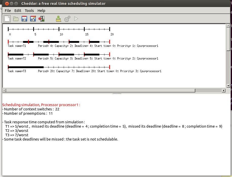
Figure 1.5 The Cheddar's main window

In the top part of this window, each resource, buffer, message and task is shown by a time line:

For a task time line:
- Each vertical red line means that the task is activated (woken up) at this time.
- Each horizontal rectangle means that the task is running at this time. The horizontal rectangle can have a task specific color. This horizontal colored rectangle can be found also on the core time line, which shows how the core is shared by the tasks of the architecture model. Task specific color can be deactivated, i.e. set to black for all tasks with the options windows.
For a resource time line:
- Each vertical blue line means that the resource is allocated by a task at this time.
- Each vertical red line means that the resource is relaesed by a task at this time.
- Each horizontal rectangle means that the resource is used by a task which is running at this time. The color of this horizontal rectangle is set with the same color used in the task time line.
For a message time line:
- Each vertical blue rectangle means that the message is sent at this time.
- Each vertical read rectangle means that the message is received at this time.
- To find the task sending or receiving a message, users have to check the core unit time line of the task time lines to find the related tasks. To produce such a display, users have to define for each message the corresponding dependencies that are used to computed the related events.
For a buffer time line:
- Each horizontal blue rectangle means that a task writes data into a buffer.
- Each horizontal red rectangle means that a task reads data from a buffer.To find the task writing or readning a data in/from the buffer, users have to check the core unit time line of the task time lines to find the related tasks. To produce such a display, users have to define for each buffer the corresponding dependencies that are used to computed the related events.

The scheduling result can also be saved in XML file. This allows user to run tools on Cheddar scheduling results. The scheduling result of Cheddar is an event table that gives for each time unit the set of events produced by the scheduling simulator. The event table is the data structure which is used by the simulator engine to perform analysis on scheduling. For each event, extra data related to the event is also stored. Here is the main produced events and their data:

Start_Of_Task_Capacity. This event is generated when a task run the fist unit of time of its capacity. The event stores the started name of the task.
End_Of_Task_Capacity. This event is generated when a task run the last unit of time of its capacity. The event stores the name of the completed task.
Write_To_Buffer. This event is generated when a task write data into a buffer. The event stores the name of the buffer, the name of the task and the size of the written data.
Read_From_Buffer. This event is generated when a task read data from a buffer. The event stores the name of the buffer, the name of the task and the size of the read data.
Running_Task. This event is generated when a task get the processor. The event stores the name of the running task, its current priority, the core on which it runs, its CRPD value and the state of the associated cache.
Task_Activation. This event is generated when a task is waking up. The event stores the name of the awoken task.
Send_Message. This event is generated when a task is sending a message. The event stores the name of the message and the name of the task.
Receive_Message. This event is generated when a task is receiving a message. The event stores the name of the message and the name of the task.
Allocate_Resource. This event is generated when a task takes a resource. The event stores the name of the resource and the name of the task.
Release_Resource. This event is generated when a task releases a resource. The event stores the name of the resource and the name of the task.
Wait_For_Resource. This event is generated when a task waits for the access to a resource. The event stores the name of the resource and the name of the task.
Address_Space_Activation. This event is generated with hierarchical scheduling such as ARINC 653 and when an address space is activated. This event stores the name of the activated address space and the activation duration, i.e. the amount of time the address space will stay activated.
Buffer_Overflow. This event is generated when running scheduling simulations with buffer and a task tries to write to a buffer which is full.
Buffer_Underflow.This event is generated when running scheduling simulations with buffer and a task tries to read from a buffer which is empty.
Context_Switch_Overhead. This event is generate when there is context switch - a change in running task.
Preemption. This event is generated whenever there is a preemptions.

Be aware that for scalability, no all events are by default generated by Cheddar. Please refer to the option windows to select which events the simulator will produce or not. Here is an example of event table produced by Cheddar:

event_table.xml : this simple event table is produced from a set of independent task scheduled with EDF. The file event_table_large.xml is similar except the size (it is a large file produced with a 200 task set).
event_table_fixed_priority.xml: this event table is produced from a fixed priority scheduler.This scheduler provide an extra information for the event Running_Task. This extra information is the current priority of the running task.
event_table_buffer.xml : this event table is produced from a set of tasks sharing a buffer.
event_table_shared_resource.xml: this event table is produced from a set of tasks sharing a PCP resource.
event_table_message.xml: this event table is produced from a set of tasks sending/receiving messages.

To get a summary of the tools provided by Cheddar, see section User Defined Scheduler.

1.2 Other available schedulers and task arrival patterns

In Cheddar, you will find several schedulers. Some of them are directly implemented into the framework; others can be defined by the user. The list below describes the currently built-in schedulers you may find in the current release:

Rate Monotonic: run the task with the smallest period first. The priority field of the tasks is ignored here. All tasks have to be periodic.
`Deadline Monotonic : run the task with the smallest static deadline first. The priority field of the tasks is ignored here. All taks have to be periodic.
Earliest Deadline First: run the task with the smallest dynamic deadline first. Tasks can be periodic or not.
Least Laxity First and Least Runtime Laxity First: run the task with the smallest laxity first. The laxity is computed according to 2 various means.
Posix 1003.1b Highest Priority First scheduler : run the task with the highest fixed priority first. Support SCHED_RR, SCHED_FIFO and SCHED_OTHERS policies. SCHED_OTHERS is a time sharing scheduler. SCHED_RR and SCHED_FIFO are policies which enforce real time scheduling. Tasks can be periodic or not. Tasks are scheduled according to the priority and the policy of the tasks. (Rate Monotonic and Deadline Monotonic use the same scheduler engine except that priorities are automaticly computed from task period or deadline). POSIX 1003.1b scheduler supports SCHED_RR, SCHED_FIFO and SCHED_OTHERS queueing policies. SCHED_OTHERS is a time sharing policy. SCHED_RR and SCHED_FIFO tasks must have priorities range from 255 to 1. Priority level 0 is reserved to SCHED_OTHERS tasks. The highiest priority level is
Maximum Urgency First scheduler [STE 91]: run the tasks according to a mixed static and dynamic priority. The task to run is the task with the highest criticality level. If two tasks have the same crititicaly level, the scheduler then chooses the one with the smallest laxity. If two tasks have the same criticality level and the same laxity, the scheduler chooses the one with the highest fixed priority.
D-over dynamic scheduler [KOR 92]: run the tasks as EDF but with a safe policy in case of transient overload.
Round robin scheduler : give the processor during a fixed delay to each task at a fixed order. It allows the use of a given quantum : in this case, a task stays on the processor until the quantum becomes exhausted.
Time sharing scheduler based on task waiting time (scheduler similar to the one provided by Linux): run the task which waits since the oldest date.
Time sharing scheduler based on cpu usage: run the task which had consumed the least cpu time.
Earliest Deadline First Energy Harvesting: a deadline oriented scheduler that takes care of the energy harvested during execution See [CHE 14].
AMC and EDF VD, which are 2 uniprocessor mixed criticality schedulers.
DAG HLFET, a multicore scheduling that is using a DAG of task dependencies. See [ADA 74].
RUN (Reduction to Uniprocessor), a optimal multicore global scheduler, both online and offline. See [REG 11].
3 implementations of the multicore global Proportionate Fair scheduling: PF, PD and PD2. See [AND 04].
EDZL, for Earliest Deadline Zero Laxity, which is a deadline oriented global multicore scheduler. See [CIR 07].
LLREF, Largest Local Remaining Execution First, which is a laxity oriented global multicore scheduler.
Hierarchical schedulers for uniprocessor architectures to support the scheduling of aperiodic tasks jointly with periodic tasks [SPR 90]:
- Hierarchical Polling Aperiodic Server, which implements a uniprocessor fixed priority scheduler with a aperiodic task server. The aperiodic task server is a periodic task running the polling protocol.
- Hierarchical Priority Exchange Aperiodic Server, which implements a uniprocessor fixed priority scheduler with a aperiodic task server. The aperiodic task server is a periodic task running the priority exchange protocol.
- Hierarchical Sporadic Aperiodic Server, which implements a uniprocessor fixed priority scheduler with a aperiodic task server. The aperiodic task server is a periodic task running the sporadic protocol.
- Hierarchical Deferrable Aperiodic Server, which implements a uniprocessor fixed priority scheduler with a aperiodic task server. The aperiodic task server is a periodic task running the deferrable protocol.
Hierarchical schedulers for uniprocessor architecture to support Time-and-Space architectures such as ARINC 653. These hierarchical scheduling has a 2 level of scheduling: 1) A scheduler inside each address space to select the task amoung the one of the related address space. 2) A scheduler at the processor level to select the address space to activate. The following protocols have been implemented:
- Hierarchical Offline: address spaces are activated/scheduled according to a offline address space scheduling stored in a XML file. This scheduler is modeling the ARINC 653 MAF partition scheduling.
- Hierarchical Cyclic: address space are activated/scheduled cyclically.
- Hierarchical Round: addres space are activated/scheduled with a round robin policy.
- Hierarchical Fixed: address spaces are activited/scheduled according to their fixed priority.

Besides the implemented scheduling protocols listed above, Cheddar provides a mean to define your own scheduling protocols. The current Cheddar's release provides examples of User-defined schedulers stored in some .sc files (see project_examples sub-directory and section VI). These scheduler examples are:

arinc.sc: modeling of an ARINC 653 partition and task scheduler
schedule_according_to_criticity.parametric-cpu.sc: schedule tasks according a task criticity level
non_preemptive_llf.sc: example of a LLF scheduler with no preemption when tasks have the same laxity value
ts.sc: the processor is given to the task which ran the least frequently.
fcfs.sc: first come/first served scheduling policy.
short.sc: schedule the shortest task first (with the smallest capacity)
dvd0.parametric-cpu.sc: Dynamic value density scheduler of the York University [ALD 98].
mllf.sc : Modified Least Laxity First scheduler with f=0.5 [OVE 97].
muf.sc : Maximum Urgency First scheduler [STE 91].

In the same way, Cheddar provides a set of built-in task models. The built-in task models are:

Aperiodic tasks: this kind of task arrives in the system at a given time (the start time, see the "Update Tasks" widget), run a job and leaves the system.
Periodic tasks: this kind of task periodically runs a job. A periodic task has a start time. The period of the task stores the fixed delay between two successive task wake-up times. See [LIU 73].
Sporadic tasks: this kind of task cyclycally runs a job. A sporadic task has a start time. The period field stores the minimum delay between two successive task wake-up times.
Poisson process tasks: this kind of task periodically runs a job. A periodic task has a start time. The period of the task stores the average delay between two successive task wake-up times. The effective delay between two wake-up times is computed with an exponential random generator.
Frame Task: this model implements the multiframe task model of [BAR 99].
Scheduling task: is planned to be used for hierarchical scheduling.
Periodic inner periodic: is a task model to specify burst of periodic release separated by a fixed amount of time. This task model is then using 2 periods: an inner period for the delay between two task releases during the burts and a second period to express the delay between two burst. See [AUD 93].
Sporadic inner periodic: this task model is similar to periodic inner periodic instead of the delay between two burts is sporadic (we specify the minimum delay between two burts). See [AUD 93].

Again, you can define your own task model with user-defined code. Examples of user-defined task provided with this Cheddar release can be found in these files:

sporadic.sc : tasks are woken up with a minimal inter-waking up period delay. The miminum delay is stored in the period field and the wake-up delay is randomly generated (exponential distribution).
random_capacity.sc : task with a randomly generated capacity.
increasing_capacity.sc : tasks with a growing capacity.
activations.sc : various task models.

1.3 Scheduling options

Figure 1.6 Scheduling options windows

The submenu "Tools/Scheduling/Options" allows you to tune the way all next scheduling simulations will be done (see Figure 1.6) :

If you push the Offsets button, the simulation engine takes care of the task offsets given at task definition time : task activations can then be delayed if you provide offset values at task definition time.
If you push the recedencies button, task scheduling will be done so that task precedencies will be met. By default, task precedencies are ignored.
If you push the Resources button, access to shared ressources will be done during simulation. By default, all shared resources are ignored.
Cheddar allows you to activate tasks randomly . If you want to do simulations with this kind of task, the simulator engive has to compute some random values. From this window, you can tune the way random activation delays are generated. A seed value can be associated with each task but you can also use only one seed for all tasks. In the two cases, you can do "predictable" or "unpredictable" simulations. If you choose "predictable" simulation, the seed will be initialized by a given value. In the other case, the seed is initialized with "gettimeofday". . Pushing the Predictable for all tasks radio button leads to take the seed value of the Option window during simulation for all tasks. If the Task specific seed radio button is pushed instead, the seed of each task is used to generate task activation delays. You should notice that by default, 0 is given to the seed value, but of course, you can choose any value. Pushing the Seed button gives you a random value for the seed.
The check button of the window on the right side allows the user to define which events will be generated into the event table at simulation time (see section Multiprocessor scheduling service).

Figure 1.7 Scheduling options windows (both feasibility and simulation)

The submenu Tools/Scheduling/Scheduling simulation allows you to tune the way the next scheduling simulation and the next feasibility test will be done (see the Figure 1.7).

Options related to which information the engine has to compute when the scheduling sequence is built are :

Pushing the Schedule all processors check button implies that the scheduling simulation will be computed on all defined processors. If this button stay unchecked, the user has to choose a given processor.
Pushing the Number of context switch implies to compute the number of context switches from the computed scheduling sequence.
Pushing the Number of preemption implies to compute the number of preemptions from the computed scheduling sequence.
Pushing the Task response time implies to compute the worst/best/average task response times from the computed scheduling sequence.
Pushing the Blocking time implies to compute the worst/best/average task blocking times on shared resources from the computed scheduling sequence.
Pushing the Run event analyzers will imply to perform the user-defined code (see section V) on the computed scheduling sequence.
The Display event table, Automatically export event table and Event table file name options are related to the computing scheduling sequence. These options allow you to save the computed scheduling into a file in a XML format or display it on the screen.

Options related to which information the feasibility tests will compute are :

Pushing the Feasibility on all processors check button implies that the feasibility tests will be computed on all defined processors. If this button stay unchecked, the user has to choose a given processor.
Pushing the Feasibility test based on the processor utilization factor will imply to compute such a test.
Pushing the Feasibility test based on worst case task response time will imply to compute such a test.