(return back to home page)

Installation procedure

How to run the tool

Demo of the basic analysis features

Installation procedure

How to run the tool

Demo of the basic analysis features

1. Create a new OSATE project.
2. Download the AADL files from here.
3. Add those AADL files in your AADL project.
4. To perform a scheduling analysis, the processor component has to be extended with few properties. Add to the cpu_leon2 component the following properties:

       PROPERTIES
          Scheduling_protocol => (rate_monotonic_protocol);
   

5. Now, we need to generate the Cheddar XML model to perform the scheduling analysis. In te windows above, you can see a screenshot of OSATE. The AADL file inserted in the AADL project is called the declarative model and no scheduling analysis can be run on the declarative model. Analysis are run on the instance model. To create an instance model from a declarative model with OSATE, in the list of component on the right side of the OSATE windows, select the top system component and open the context menu (with the right mouse button), then select the "instanciate" menu item. The instance model appears in the middle of the OSATE windows. From this instance model, we can then generate the Cheddar XML model by selecting the root component of the instance model and pushing the Left Cheddar button. The generated Cheddar XML model is then saved in a location given by the dialog windows opened when the transforamtion is over.
   
   
   
   
   
6. We can now call Cheddar with the generated Cheddar XML file. The window of Cheddar is displayed there:
   
   
   
   
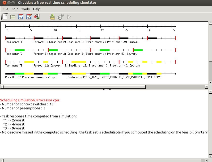
   The top part of this window (in gray in the figure) displays the time lines computed during scheduling simulation. The bottom part of this window displays numeric analysis results.
   
   From the menu Tools and for a given architecture model, we can perform 3 types of analysis with Cheddar:
   • We can use simulation tools to compute the scheduling of a task set, and then, from such scheduling, to compute various performance criteria (worst/average/best response times, missed deadlines, blocking time on shared resources, deadlocks, ...).
   • We can also call various feasibility tests that allow the designers to check deadlines without computing the scheduling of the task set.
   • If the previous tools have shown that some deadlines cannot be met, we can also improve the architecture model by various means : priority assignments, task partitionning, task clustering, ...
   
   
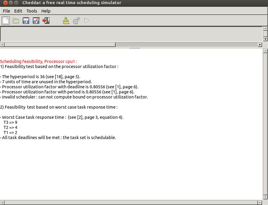
   Under the menu, some buttons allow you to quickly access to a summary of those Cheddar analysis features (all analysis features can be accessed by the Tools menu). Indeed, the button starts a scheduling simulation and the button computes a sample of feasibility tests for a basic periodic task set. Basically, the button computes worst case task response time following the Joseph et Pandia [wiki:references (Joseph 86)] method extended for any Deadline and classical CPU bound tests. Again, for specific feasibility tests (e.g. transactions), see the Tools menu.
   
   The two figures below show a screenshot of Cheddar for the model edited in section I.2, and for results produced by buttons and . We can see there worst case response times computed by the Joseph and Pandia (Joseph 86) feasibility test and also by the scheduling simulation on the hyper-period. Feasibility tests on cpu utilization factor cannot be applied there as the tool cannot be sure that priorities have been assigned according to Rate Monotonic. To apply this test, one must change the scheduling policy of the core1 component with the Rate_Monotonic_Protocol value.
   
   We can also notice in the time lines that red rectangles show task release times, black rectangles show when tasks are running. Many other display options exist there and can be modified by the Tools/Scheduling/Scheduling Options menu (for example to display a different color for each task).
   
   
   
   
   
   
   
   
7. Compute the scheduling simulation of this thread set with Cheddar. From this simulation, compute with Cheddar the response times of the threads.
8. Compute theoretical worst case thread response times, always with Cheddar but with the feasbility tests button.
9. Explain why we have different response times for each thread?
10. Update the Scheduling_protocol property for subcomponent cpu with value posix_1003_highest_priority_first_protocol
11. Do again the questions 6 upto 8.

(return back to home page)