Cheddar is a free real time scheduling framework. Cheddar is designed for checking task temporal constraints of a real time application/system. It can also help you for quick prototyping of real time schedulers. Finally, it can be used for educational purpose. Cheddar is a free software, and you are welcome to redistribute it under certain conditions; See the GNU General Public License for details. The Cheddar project was started in 2002 by the LISyC Team, University of Western Britanny. Since 2008, Ellidiss technologies also contributes to the development of Cheddar and provides industrial support.

WARNING : this user's guide supposes that you have a minimum background on real time applications/systems and real time scheduling. If it's not your case, take a look on this link which includes some very basic articles or book references. This link also provides a description of the analytical methods implemented into Cheddar and gives some publications that show how to use Cheddar.

• I. Basic scheduling simulation features and feasibility tests
• I.1 First step : a simple scheduling simulation
• I.2 Other available schedulers and task arrival patterns
• I.3 Scheduling options
• II. About Cheddar project files (XML and AADL files)
• III. Summary of the Cheddar command line
• IV. Scheduling with task dependencies
• IV.1 Shared resources analysis tools
• IV.2 Task precedencies
• IV.2.1 Editing Task precedencies
• IV.2.2 How to transform a dependent task set into an undependent task set : the Chetto/Blazewicz modification rules
• IV.2.3 Computing end to end response time : the Holistic approach
• IV.3 Buffer analysis tools
• IV.4 Message scheduling services
• V. Multiprocessor scheduling services
• VI. User-defined simulation code : how to run simulations of specific systems
• VI.1 Examples of user-defined schedulers
• VI.1.1 Low-level statements versus High-level statements
• VI.1.2 User-defined scheduler built with User's defined Task Parameters
• VI.2 Scheduling with user-defined task arrival patterns
• VI.3 Running a simulation with a user-defined scheduler
• VI.4 Looking for user-defined properties during a scheduling simulation
• VI.5 List of predefined variables and available statements for user-defined code
• VII. Summary of Cheddar's editor menus and sub-menus

I. Basic scheduling simulation features and feasibility tests for independent tasks

In this chapter, you find a description of the most important scheduling and feasibility services provided by Cheddar in the case of independent tasks.

I.1 First step : a simple scheduling simulation

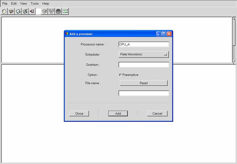
Cheddar provides tools to check temporal constraints of real time tasks. These tools are based on classical results from real time scheduling theory. Before calling such tools, you have to define a system which is mainly composed of several processors and tasks. To define a processor, choose the "Edit/Update processors" submenu. The window below is then displayed :

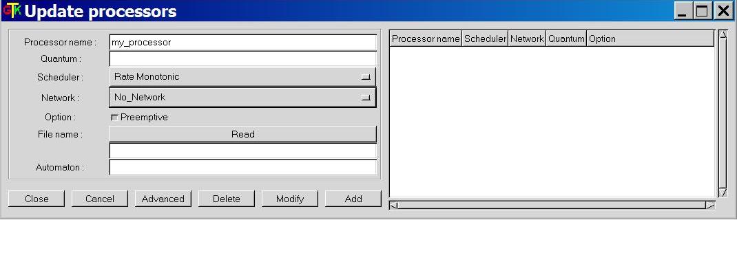
A processor is defined by the following fields (see Figure 1.1) :

• A name. An address space name can be any combination of literal characters including underscore. Space is forbidden. Each address space name has to be unique.
• A processor name. This is the processor which hosts the address space.
• Some fields related to the size of the address space memory : the text memory size, the heap memory size, the stack memory size and the data memory size. The fields related to memory size will be used in the next Cheddar's release in order to perform a global memory analysis.
• As for the processor objects, an address space may include a scheduler (in the context of hierarchical scheduling algorithms for example). In this case, you can also specify a scheduler name, its quantum, a file name if the scheduler is a user-defined one and finally the option if your scheduler is preemptive.

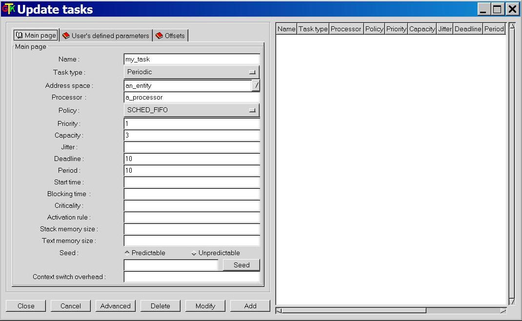
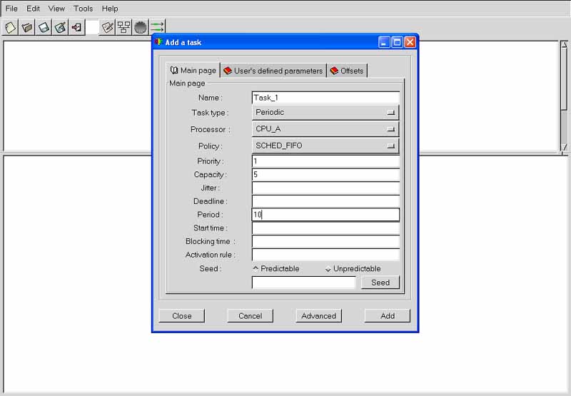
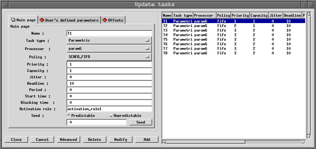
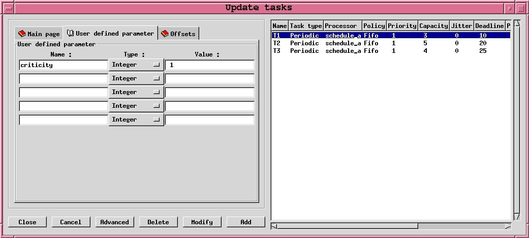
Let see now, how to define a task, the last feature required to perform the most simpliest performance analysis. Choose the "Edit/Update tasks" submenu. The window of Figure 1.3 is then displayed. This window is composed of 3 sub-windows : the "main page", the "offset page" and the "user's defined parameters page". The main page contains the following information :

1. At least, a task is defined by a name (the task name should be unique), a capacity (bound on its execution time) and a place to run it (a processor name and an address space name). The other parameters are optional but can be required for a particular scheduler
2. A type of task . It describes the way the task is activated. An aperiodic task is only activated once. A periodic task is activated many times and the delay between two activations is a fixed one. A poisson process task is activated many times and the delay between two activations is a random delay : the random law used to generated these delays is an exponential one (poisson process). a sporadic task is a task which is activated many times with a minimal delay between two succesive activatiosn. If the task type is "user-defined", the task activation law is defined by the user (see section VI.2 of this user's guide).
3. The period. It is the time between two task activations. The period is a constant delay for a periodic task. It's an average delay for a poisson process task. If you have selected a processor that owns a Rate Monotonic or a Deadline Monotonic scheduler, you have to give a period for each of its tasks.
4. A start time. It is the time when the task arrives in the system (its first activation time).
5. A deadline. The task must end its activation before its deadline. A deadline is a relative information : to get the absolute date at which a task must end an activation, you should add the time when the task was awoken/activated to the task deadline. Warning : the deadline must be equal to the period if you define a Rate Monotonic scheduler.
6. A priority and a policy. These parameters are dedicated to the POSIX 1003.1b/Highest Priority First scheduler. Priority is the fixed priority of a task. Policy can be SCHED_RR, SCHED_FIFO or SCHED_OTHERS and describes how the scheduler chooses a task when several tasks have the same priority level. Warning : the priority and the policy are ignored by a Rate Monotonic and a Deadline Monotonic scheduler.
7. A jitter. The jitter is a maximum lateness on the task wake up time. This information can be used to express task precedencies and to applied method such as the Holistic task response time method.
8. A blocking time. It's a bound on shared resource waiting time. This delay could be set by the user but could also be computed by Cheddar if you described how shared resources are accessed.
9. An activation rule. The name of the rule which defines the way the task should be activated. Only used with user-defined task. (see section VI.2 for details).
10. A criticality level . The field indicates how the task is critical. Currently used by the MUF scheduler or any user-defined schedulers.
11. A seed . If you define a poisson process task or a user-defined task, you can set here how random activation delay should be generated (in a deterministic way or not). The "Seed" button proposes you a randomly generated seed value but of course, you can give any seed value. This seed value is used only if the Predictable button is pushed. If the Unpredictable button is pushed instead, the seed is initialized at simulation time with "gettimeofday".
12. The text memory size and stack memory size. The fields related to task memory size will be used in the next Cheddar's release in order to perform memory requirement analysis.

Finally, the third page (the "User's defined parameters" page) contains task parameters (similar to the deadline, the period, the capacity ...) used by user-defined schedulers. With this page, a user can define new task parameters. A user-defined task parameter has a value, a name and a type. The types currently available to defined user-defined task parameters are : string, integer boolean and double.

Warning : when you create tasks, in most of cases, Cheddar does not check if your task parameters are erronous according to the scheduler you previously selected : these checks are done at task analysis/scheduling. Of course, you can always change task and processor parameters with "Edit/Update and "Edit/Duplicate" menus.

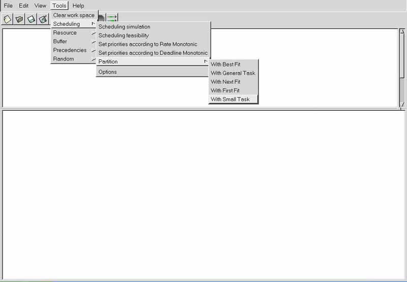
When tasks and processors are defined, we can start the task analysis. Cheddar provides two kind of analysis tools :

1. Feasibility analysis tools : these tools compute much information without scheduling the set of tasks. Equation references used to compute this feasibility information are always provided with the results. Feasibility services are provided for tasks and buffers.
2. Simulation analysis tools : With these tools, scheduling has to be computed first. When the scheduling is computed (of course, this step can be long to proceed ...), the resulting scheduling is drawn in the top part of the window and information is computed and displayed in the bottom part of the window. Information retrieved here is only valid in the computed scheduling.The simpliest tools provided by Cheddar check if a set of tasks meet their temporal constraints. Simulation services are also provided for other resources (for buffers for instance).

All these tools can be called from the "Tools" Menu and from some toolbar Buttons :

• From the submenu "Tools/Scheduling/Customized scheduling simulation", the scheduling of each processor is drawn on the top of the Cheddar main window (see below). From the drawn scheduling, missed deadlines are shown and some statistics are displayed (number of preemption for instance).
  
• From the submenu "Tools/Scheduling/Customize scheduling feasibility", response time, base period and processor utilization level are computed and displayed on the bottom of the Cheddar main window (see Figure 1.4).

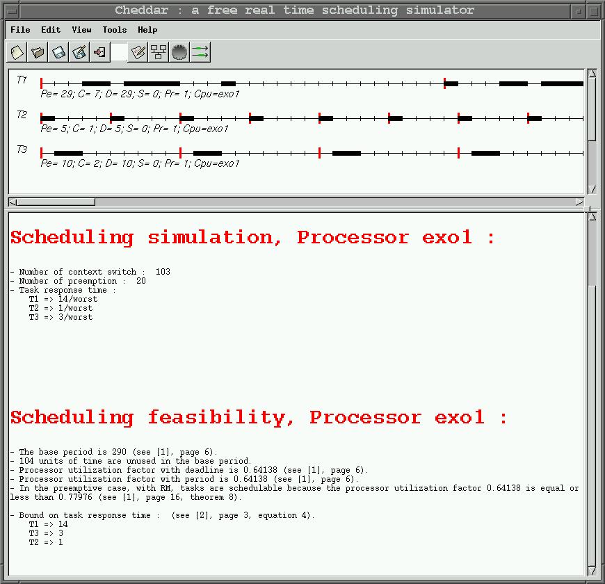
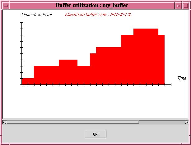
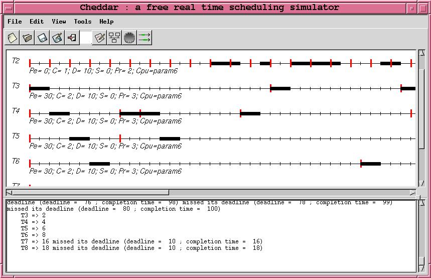
In the top part of this window, each resource, buffer, message and task is shown by a time line :

1. For a task time line :
   • Each vertical red line means that the task is activated (woken up) at this time.
   • Each black rectangle means that the task is running at this time.
2. For a resource time line :
   • Each vertical blue line means that the resource is allocated by a task at this time.
   • Each black rectangle means that the resource is used by the task which is running at this time.
3. For a message time line : each black rectangle means that the message is beeing transmitted by the network.
4. For a buffer time line :
   • Each write rectangle means that a task writes data into a buffer.
   • Each red rectangle means that a task reads data from a buffer.

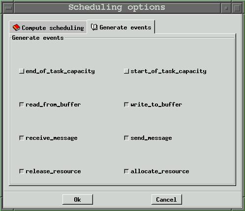
The scheduling result can also be saved in XML file. This is particulary usefull if you do not want to use the Cheddar Machine-Man-Interface. For example, the computed scheduling as an event table. The event table is the data structur used by the simulator engine to perform analysis on scheduling. The event produced by the simulator are : Start_Of_Task_Capacity, End_Of_Task_Capacity, Write_To_Buffer, Read_From_Buffer, Running_Task, Task_Activation, Send_Message, Receive_Message, Allocate_Resource, Release_Resource and Wait_For_Resource. In a XML event table file, an event Each event is exported with the time the event occurs. For each event, some extra data related to the event can also be exported :

• Start_Of_Task_Capacity. This event is generated when a task run the fist unit of time of its capacity. The exported information is the name of the task.
• End_Of_Task_Capacity. This event is generated when a task run the last unit of time of its capacity. The exported information is the name of the task.
• Write_To_Buffer. This event is generated when a task write data into a buffer. The exported information is the name of the buffer, the name of the task and the size of the written data.
• Read_From_Buffer. This event is generated when a task read data from a buffer. The exported information is the name of the buffer, the name of the task and the size of the read data.
• Running_Task. This event is generated when a task get the processor. The exported information is the name of the running task.
• Task_Activation. This event is generated when a task is awoken. The exported information is the name of the awoken task.
• Send_Message. This event is generated when a task is sending a message. The exported information is the name of the message and the name of the task.
• Receive_Message. This event is generated when a task is receiving a message. The exported information is the name of the message and the name of the task.
• Allocate_Resource. This event is generated when a task takes a resource. The exported information is the name of the resource and the name of the task.
• Release_Resource. This event is generated when a task releases a resource. The exported information is the name of the resource and the name of the task.
• Wait_For_Resource. This event is generated when a task waits for the access to a resource. The exported information is the name of the resource and the name of the task.

• event_table.xml : this simple event table is produced from a set of independent task scheduled with EDF. The file event_table_large.xml is similar except the size (it is a large file produced with a 200 task set).
• event_table_fixed_priority.xml : this event table is produced from a fixed priority scheduler.This scheduler provide an extra information for the event Running_Task. This extra information is the current priority of the running task.
• event_table_buffer.xml : this event table is produced from a set of tasks sharing a buffer.
• event_table_shared_resource.xml : this event table is produced from a set of tasks sharing a PCP resource.
• event_table_message.xml : this event table is produced from a set of tasks sending/receiving messages.

To get a summary of the tools provided by Cheddar, see section VI .

I.2 Other Available schedulers and task arrival patterns

• Rate Monotonic : run the task with the smallest period first. The priority field of the tasks is ignored here. All tasks have to be periodic.
• Deadline Monotonic : run the task with the smallest static deadline first. The priority field of the tasks is ignored here. All taks have to be periodic.
• Earliest Deadline First : run the task with the smallest dynamic deadline first. Tasks can be periodic or not.
• Least Laxity First : run the task with the smallest laxity first. The laxity is computed according to the task deadline. Tasks can be periodic or not.
• POSIX 1003.1b scheduler : run the task with the highest fixed priority first. Support SCHED_RR, SCHED_FIFO and SCHED_OTHERS policies. SCHED_OTHERS is a time sharing scheduler. SCHED_RR and SCHED_FIFO are policies which enforce real time scheduling. Tasks can be periodic or not. Tasks are scheduled according to the priority and the policy of the tasks. (Rate Monotonic and Deadline Monotonic use the same scheduler engine except that priorities are automaticly computed from task period or deadline). POSIX 1003.1b scheduler supports SCHED_RR, SCHED_FIFO and SCHED_OTHERS queueing policies. SCHED_OTHERS is a time sharing policy. SCHED_RR and SCHED_FIFO tasks must have priorities range from 255 to 1. Priority level 0 is reserved to SCHED_OTHERS tasks. The highiest priority level is
• Maximum Urgency First scheduler [STE 91] : run the tasks according to a mixed static and dynamic priority. The task to run is the task with the highest criticality level. If two tasks have the same crititicaly level, the scheduler then chooses the one with the smallest laxity. If two tasks have the same criticality level and the same laxity, the scheduler chooses the one with the highest fixed priority.
• D-over dynamic scheduler [KOR 92] : run the tasks as EDF but with a safe policy in case of transient overload.
• Round robin scheduler : give the processor during a fixed delay to each task at a fixed order. It allows the use of a given quantum : in this case, a task stays on the processor until the quantum becomes exhausted.
• Time sharing scheduler based on task waiting time (scheduler similar to the one provided by Linux) : run the task which waits since the oldest date.
• Time sharing scheduler based on cpu usage : run the task which had consumed the least cpu time.

• arinc.sc : modeling of an ARINC 653 partition and task scheduler
• schedule_according_to_criticity.parametric-cpu.sc : schedule tasks according a task criticity level
• non_preemptive_llf.sc : example of a LLF scheduler with no preemption when tasks have the same laxity value
• ts.sc : the processor is given to the task which ran the least frequently.
• fcfs.sc : first come/first served scheduling policy.
• short.sc : schedule the shortest task first (with the smallest capacity)
• dvd0.parametric-cpu.sc : Dynamic value density scheduler of the York University [ALD 98].
• mllf.sc : Modified Least Laxity First scheduler with f=0.5 [OVE 97].
• muf.sc : Maximum Urgency First scheduler [STE 91].

In the same way, Cheddar provides a set of built-in task arrival patterns. The built-in task arrival patterns are :

• Aperiodic tasks : this kind of task arrives in the system at a given time (the start time, see the "Update Tasks" widget), run a job and leaves the system.
• Periodic tasks : this kind of task periodically runs a job. A periodic task has a start time. The period field (see the "Update Tasks" widget) stores the fixed delay between two successive task wake-up times.
• Poisson process tasks : this kind of task periodically runs a job. A periodic task has a start time. The period field (see the "Update Tasks" widget) stores the average delay between two successive task wake-up times. The effective delay between two wake-up times is computed with an exponential random generator.

• sporadic.sc : tasks are woken up with a minimal inter-waking up period delay. The miminum delay is stored in the period field and the wake-up delay is randomly generated (exponential distribution).
• random_capacity.sc : task with a randomly generated capacity.
• increasing_capacity.sc : tasks with a growing capacity.
• activations.sc : various task models.

I.3 Scheduling options.

• If you push the "Offsets" button, the simulation engine takes care of the task offsets given at task definition time : task activations can then be delayed if you provide offset values at task definition time.
• If you push the "Precedencies" button, task scheduling will be done so that task precedencies will be met. By default, task precedencies are ignored.
• If you push the "Resource" button, access to shared ressources will be done during simulation. By default, all shared resources are ignored.
• Cheddar allows you to activate tasks randomly . If you want to do simulations with this kind of task, the simulator engive has to compute some random values. From this window, you can tune the way random activation delays are generated. A seed value can be associated with each task but you can also use only one seed for all tasks. In the two cases, you can do "predictable" or "unpredictable" simulations. If you choose "predictable" simulation, the seed will be initialized by a given value. In the other case, the seed is initialized with "gettimeofday". . Pushing the "Predictable for all tasks" radio button leads to take the seed value of the Option window during simulation for all tasks. If the "Task specific seed" radio button is pushed instead, the seed of each task is used to generate task activation delays. You should notice that by default, 0 is given to the seed value, but of course, you can choose any value. Pushing the "Seed" button gives you a random value for the seed.
• The check button of the window on the right side allows the user to define which events will be generated into the event table at simulation time (see section V).

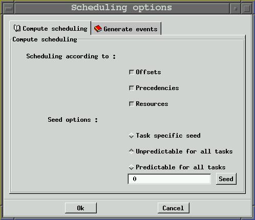
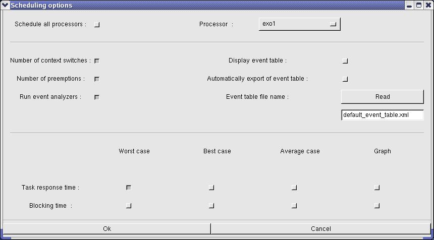
Options related to which information the engine has to compute when the scheduling sequence is built are :

• Pushing the "Schedule all processors" check button implies that the scheduling simulation will be computed on all defined processors. If this button stay unchecked, the user has to choose a given processor.
• Pushing the "Number of context switch" implies to compute the number of context switches from the computed scheduling sequence.
• Pushing the "Number of preemption" implies to compute the number of preemptions from the computed scheduling sequence.
• Pushing the "Task response time " implies to compute the worst/best/average task response times from the computed scheduling sequence.
• Pushing the "Blocking time" implies to compute the worst/best/average task blocking times on shared resources from the computed scheduling sequence.
• Pushing the "Run event analyzers" will imply to perform the user-defined code (see section V) on the computed scheduling sequence.
• The Display event table, Automatically export event table and Event table file name options are related to the computing scheduling sequence. These options allow you to save the computed scheduling into a file in a XML format or display it on the screen.

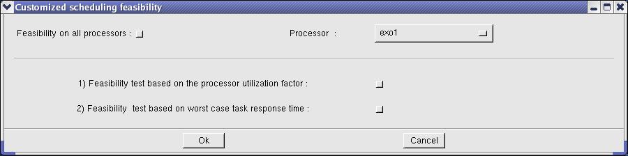
Options related to which information the feasibility tests will compute are :

• Pushing the "Feasibility on all processors" check button implies that the feasibility tests will be computed on all defined processors. If this button stay unchecked, the user has to choose a given processor.
• Pushing the "Feasibility test based on the processor utilization factor" will imply to compute such a test.
• Pushing the "Feasibility test based on worst case task response time" will imply to compute such a test.

II. About Cheddar project files (XML and AADL files).

Information stored during a simulation can be saved into project files. A project file is a XML file defined by this DTD. By the way, you do not need a deep understanding of the layout of cheddar project files except if you want to edit project files by hand. If so, you should check if your project files are correctly structured by the tool xml2xml (xml2xml just reads, parses and displays the content of a XML Cheddar project file on the screen ).

All Cheddar XML files can be displayed with an Internet Browser if you put the following XSLT file and the following.CSS file in the directory hosting your XML Cheddar files. To do so, you should use a recent release of Internet Explorer (version 6.0 or later), Netscape (version 7.0 or later) or Mozilla (version 1.0 or later).

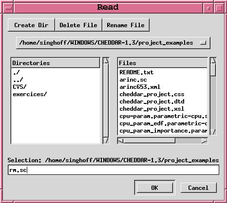
From Cheddar, there are two ways to load a project file :

• First, a project file can be loaded from the "File/Open XML project" submenu. Just click on the Open button, and give the file name of your project.
• Second, a project can be loaded from the command line. For instance, to start Cheddar and load the project file my_project.xml, just do :

  my_shell$cheddar my_project.xml
  

Saving a project can be done with the same "File" menu.

Cheddar can also import AADL specification [SAE 04]. This service can be accessed through the submenu "File/AADL/Import AADL". In the same way, an XML project can be exported towards an AADL specification (see the "File/AADL/Export AADL" sub-menu). As with XML files, you can launch Cheddar with an AADL file given from the command line. To launch Cheddar and automatically read the foo.aadl AADL specification file, do :

my_shell$cheddar -a foo.aadl

Finally, XML or AADL files can be loaded from any directory and a project can be saved in several project files. For example, to load a project saved in two AADL files called bar1.aadl and bar2.aadl, which are stored in the directory /home/foo, you must use the following command-line :

my_shell$cheddar -I/home/foo -a bar1.aadl bar2.aadl

III. Summary of the Cheddar command line.

my_shell$cheddar [switches] foo1 foo2 ...

where foo1 foo2 can be an unique XML file or one or several AADL files.

Switches can be :

• -u get the help.
• -l select a language : "fr" for français; "en" for english Default language is English.
• -a the file names given to cheddar contain AADL descriptions instead of an XML file Only one XML file can be provided to Cheddar but several AADL files can be sent to Cheddar.
• -I directory-name : gives an extra directory name where to look for XML or AADL files. By default, Cheddar only looks for project files into the Cheddar's current directory.
• -d activate Cheddar's debug mode : provides extra information on the way Cheddar works.
• -c put the current Cheddar's configuration at the screen : usefull to check that the Cheddar binary you're using is correctly tuned according to the models you would like to analyze.

IV. Scheduling with task dependencies

This chapter describes services provided by Cheddar when the system you want to study has task dependencies. By task dependencies, we mean resources shared by several tasks (ex : semaphores) or precedency relationships between several tasks (due to buffer access or message exchange or also constraints between the end of a task and the start of another one).

IV.1 Shared resources analysis tools.

1. An unique name.
2. An initial value/state (simular to a semaphore initial value). During a scheduling simulation, at a given time, if a resource value is equal or less than zero, the requesting tasks are blocked until the semaphore/shared resource is released. An initial value equal to 1 allows you to design a shared resource that is initially free and that can be used by only one task at a given time.
3. A protocol. Currently, you can choose between PCP (for Priority Ceiling Protocol), PIP (for Priority Inheritance Protocol) or "No protocol". With PCP or PIP, accessing shared resources may change task priorities [SHA 90]. The "No protocol" just means that no task prioriy will be changed at accessing the shared resource.
4. A processor name. Each shared resource has to be hosted by a given processor.
5. Finally, we must give information on tasks that need the resource. Tasks hold resources in critical section. Each critical section has to be defined by :
   • The task name requiring the shared resource.
   • The start time of the critical section.
   • The end time of the critical section.
   Of course, you can define several critical sections for a given task of a given shared resource.

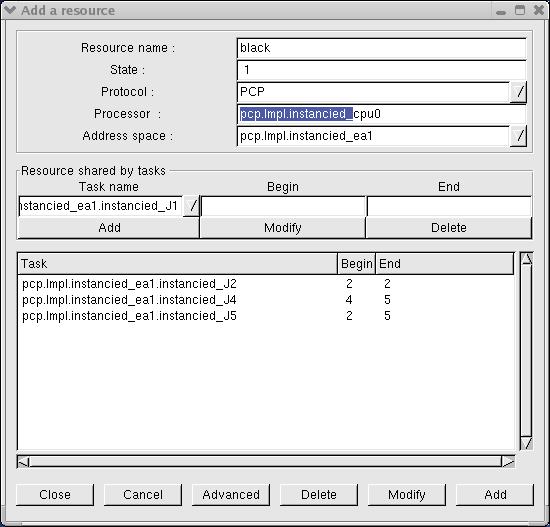
By default, shared resources analysis tools are not included in the scheduling simulation engine of Cheddar. See "Tools/Scheduling/Options" if you want to take care of shared resources during scheduling simulation and if you want to display shared resources time line. Blocking time on shared resources can be computed from scheduling simulation analysis if scheduling simulation is invoked from the sub-menu "Tools/Scheduling/Scheduling Simulation".

Finally, from the "Tools/Resources/Blocking time" sub-menu, you will find services to compute bounds on blocking time of each tasks. These bounds are computed without assumption on the scheduling actually generated for the analyzed system. To compute blocking time bound, shared resources have to used PCP or PIP protocols.

IV.2 Task precedencies.

IV.2.1 Editing Task precedencies

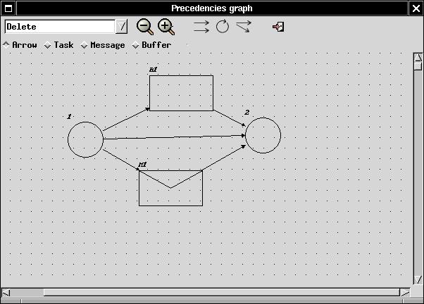
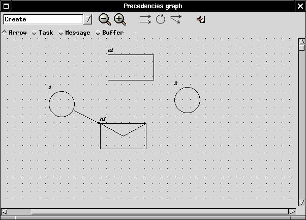
To create a dependency, you may open the "Precedencies Graph" window by clicking on the appropriate icon on the main Cheddar window. By the way, all Cheddar objects are imported in this window. All items are represented by geometrical forms :

• Tasks -> circles.
• Messages -> rectangles.
• Buffers -> enveloppes.

If there is no item on the canvas, it means that you have not created any dependency before... So you can create one by entering in "Create" mode (on the top left corner) and selecting "Task" on the radio button. After that, create a task by clicking on the canvas, then a popup appears asking you to create a new or import one task from Cheddar (cf section I). It's the same succession of operations to create other types of items (buffers and messages).

Figure 3.2 Add a new task dependency

IV.2.2 How to transform a dependent task set into an undependent task set : the Chetto/Blazewicz modification rules

IV.2.3 Computing end to end response time : the Holistic approach

IV.3 Buffer analysis tools.

Cheddar allows you to define buffers shared by tasks. If you want to define a buffer, a processor, an address space and a least one task have to be defined before. A buffer can be added to a Cheddar project with the submenu "Edit/Update buffers". The window below is then displayed :

Figure 3.4 Add a new buffer

• A buffer has a unique name, size and is hosted by a processor and an address space.
• A queueing system model is assigned to each buffer. This queueing system model describes the way buffer read and write operations will be done at simulation time. This information is also used to apply buffer feasibility tests.
• A list of tasks which access to the buffer (read or write operations). Two type of tasks can access a buffer : producers and consumers . We suppose that a producer/consumer writes/reads a fixed size of information in the buffer. For each producer or consumer, the size of the information produced or consummed have to be defined. The time of the read/write operation is also given : this time is relative to the task capacity (eg. if T2 consumes a message at time 2, it means that the message will be removed from the buffer when T2 run the 2nd unit of time of its capacity).

Like tasks, two kinds of tools can be invoked by the user from a buffer : simulation and feasibility tools. At first, the simulation of the task scheduling can help the user to see how the buffer is filled or not with messages (see "Tools/Buffer/Buffer simulation" submenu). In this case, a scheduling simulation must be previously run. The result is then displayed in a window as below :

Buffer Feasibility mainly consists of computing buffer bounds. Bounds computed here suppose that each task that is defined as "producer", produces one message per periodic activation. In the same manner, each "consumer" extracts one message during each of its periodic activation.

Figure 3.5 Display buffer utilization factor computed from scheduling simulation

The picture contains the buffer utilization level for each time.
Second, the feasibility tool provides a way to compute bounds on buffer utilization level. At the time we write this User's guide, bounds do not depend on the type of the scheduler. Bounds can be computed from the "Tools/Buffer/Buffer feasibility" submenu.

IV.4 Message scheduling services.

V. Multiprocessor scheduling services.

Multiprocessor system is good for heavy computing demands. It is sometimes the only way to provide sufficient processing power to meet critical real-time deadlines. In general multiprocessor systems are also more reliable than uni-processor systems. Scheduling of multiprocessor systems is proven to be a NP-hard (Non-deterministic Polynomial-time) problem [LEU 82]. The complexity class NP is the set of decision problems that can be solved by a non-deterministic machine in polynomial time. The complexity theory is part of the theory of computation dealing with the resources required during computation to solve a given problem. The most common resources are time (how many steps does it take to solve a problem) and space (how much memory does it take to solve a problem). Other resources can also be considered, such as how many parallel processors are needed to solve a problem in parallel. There are many scheduling heuristics to solve this. Rate-monotonic scheduling is good for numerous reasons: Rate-monotonic algorithm is optimal for fixed priority assignment of periodic tasks on a processor so it’s easy to design predictable real-time system. Also it’s easy to implement and it takes minimal scheduling overhead.

Cheddar has four algorithms: RMNF, RMFF, RMBF, RMST and RMGT. Each of these are off-line schemes, so the entire task set must be known before starting task assignment. Bounds for functions are calculated using .

Rate-Monotonic-Next-Fit [SON 93]

Upper bound for this algorithm is 2.67. Tasks are sorted in non-decreasing order of periods. Then tasks are placed on processors, according to the IP Condition (Increasing Period). The first task is placed on the first processor. Then the second task is placed on the first processor, if it meets the IP Condition. Otherwise it is placed on a new processor. This continues until all tasks are scheduled.

Rate-Monotonic-First-Fit [SON 93]

The upper bound for this algorithm is 2.33 [SON 93] (original study by Liu and Dhall had a wrong bound of 2.23). Tasks are sorted in non-decreasing order of periods. The IP Condition is used to verify teh schedulability of tasks on processors. The first task is placed on the first processor. Then the second task is placed on the first processor, if it meets the IP Condition. Otherwise it is placed on a new processor. The third task is tried to be placed on the first processor according to the IP Condition. If it does not meet the condition, the task is tried to be placed on the second processor. Otherwise a new processor is selected for the third task…

Rate-Monotonic-Best-Fit [SON 93]

The upper bound for this algorithm is 2.33. Tasks are sorted in non-decreasing order of periods. The first task is placed on the first processor. For the second task, the function checks all processors, whether they meet the IP Condition. For processors that satisfy the condition, the algorithm checks the number kj of tasks already assigned to each processor j, and computes Uj, the total utilization of the kj tasks. And the task is assigned to the processor that has the smallest value. If the condition is not met, a new processor is selected for the task.

Rate-Monotonic Small-Tasks [BUR 94]

The upper bound for RMST is , a = max Ui, i = 1,…,K and U is utilization of all tasks. Tasks are sorted in increasing Si. Si = log2(Ti). The main idea of RMST is to minimize the value of b for each processor. ß = max Si – min Si, 1= i =K.

Rate-Monotonic General-Tasks [BUR 94]

The upper bound for RMGT is 1.75. RMGT uses the RMST algorithm for task s = 1/3 and First-Fit heuristics for the rest of the tasks.

Example of use :

1. First, Define processors for tasks. They have to be of Rate Monotonic type.
   
   
   
   
2. Second, Define tasks (host tasks on any processor)
   
   
   
   
3. Third, compute partitioning :
   
   
   
   

VI. User-defined simulation code : how to run simulations of specific systems.

Usual feasibility tests are limited to only few task models (mainly periodic tasks) and to only few schedulers. When an application built with a particular task activation pattern or scheduled with a particular scheduler has to be checked, feasibility tests are not necessarily available. In this case, the only solution consists in analyzing the scheduling simulation. Cheddar allows the user to design and easily build framework extensions to do simulation of user-defined schedulers or task activation patterns. By easy, we mean quickly write and test framework extensions without a deep understanding of the framework design and of the Ada language. We propose the use of a simple language to describe framework extensions. Framework extensions are interpreted at simulation time. As a consequence, they can be changed and tested without recompiling the framework itself.


Figure 5.1 How a user-defined code is run by the scheduling engine

Figure 5.1 gives an idea on the way the simulation engine is implemented in the framework. Running a simulation with Cheddar is a three-step process.

The first step consists of computing the scheduling : we have to decide which events occur for each unit of time. Events can be allocating/releasing shared resources, writing/reading buffers, sending/receiving messages and of course running a task at a given time. At the end of this step, a table is built which stores all the generated events. The event table is built according to the XML description file of the studied application and according to a set of task activation patterns and schedulers. Usual task activation patterns and schedulers are predefined in the Cheddar framework but users can add their own schedulers and task activation patterns.

In the second step, the analysis of the event table is performed. The table is scanned by "event analyzers" to find properties on the studied system. At this step, some standard information can be extracted by predefined event analyzers (worst/best/average blocking time, missed deadlines ..) but users can also define their own event analyzers to look for ad-hoc properties (ex : synchronization constraints between two tasks, shared resources access order, ...). The results produced during this step are XML formatted and can be exported towards other programs.

Finally, the last step consists of displaying XML results in the Cheddar main window (see Figure 1.4).

VI.1 Defining new schedulers or task activation patterns.

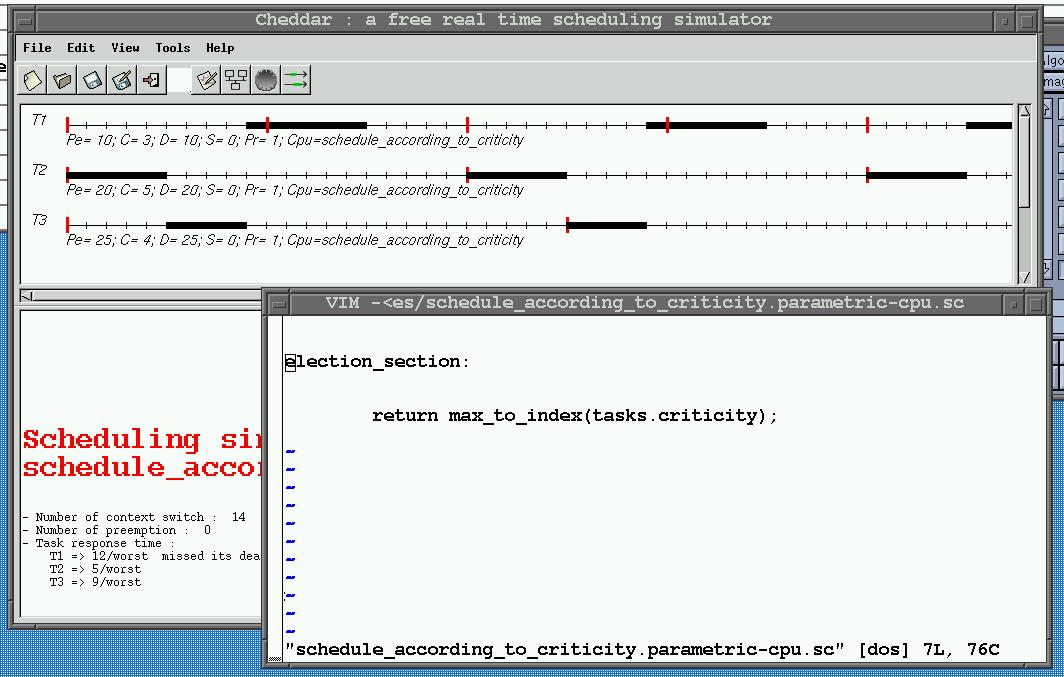
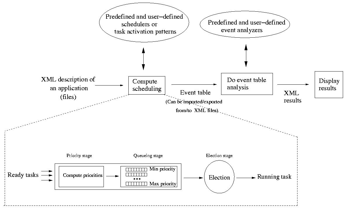
Now, let's see how user-defined schedulers or task activation patterns can be added into the framework. Basically, all tasks are stored in a set of arrays. Each array stores a given information for all tasks (ex : deadline, capacity, start time, ...). The job of a scheduler is to find a task to run from a set of ready tasks. To achieve this job, Cheddar models a scheduler with a 3 stages pipe-line which is similar to the POSIX 1003.1b scheduler (see [GAL 95]). These 3 stages are :

1. The priority stage. For each ready task, a priority is computed.
2. The queueing stage. Ready tasks are inserted into different queues. There is one queue per priority level. Each queue contains all the ready tasks with the same priority value. Queues are managed like POSIX scheduling queues : if a quantum is associated with the scheduler, queues work like the SCHED_RR scheduling queueing policy. Otherwise, the SCHED_FIFO queueing policy is applied.
3. The election stage. The scheduler looks for the non empty queue with the highest priority level and allocates the processor to the task at the head of this queue. The elected task keeps the processor during one unit of time if the designed scheduler is preemptive or during all its capacity if the scheduler is not preemptive.

Defining a new scheduler is simply giving piece of code for some of the pipe-line stages we described above. Each of these stages can be defined by a user without the need to have a deep knowledge of the way the scheduling simulator works. User-defined schedulers are stored in text files. These files are organized in several sections :

• The start section. In this section, you may declare variables needed to schedule your tasks. Many variables are already predefined in Cheddar. Some of them are those defined at task/processor/buffer/message definition (ex : period, deadline, capacity ...). This set of predefined variables can be extended with the "Edit/Update Tasks" submenu (see user-defined parameters). The others are managed by the simulator engine and describe the state of tasks/processors/buffers/messages at simulation time. See section VI.5 for a list of all predefined variables. All variables used in a scheduler should have a type. The framework provides two type families : scalar types and arrays. One can define variable with scalar type of double, integer, boolean, string and also of random (a random is a type which allows the user to generate ramdom values). An array is a type which stores one scalar data per task, message, buffer or shared resource. Arrays are declared as usual Ada Table. Vectorial operations can be done on this kind of variable.
• The priority section. The section contains the code necessary to compute task priorities. The code given here is called each time a scheduling decision has to be made (at each unit of time for preemptive scheduler and when a task has run during all its capacity for non preemptive scheduler). The code given here can be composed of many differents statements described in section VI.5
• The election section. This section just decides which task should receive the processor for next units of time. This section should only contain one return statement.
• The task activation section. This section describes how tasks could be activated during a simulation. In Cheddar, 3 kinds of tasks exists : aperiodic tasks which are activated only one time and periodic or poissons process tasks which are activated several times. In the case of periodic tasks, two successive task activations are delayed by an amount of fixed time called period. In the case of poisson process tasks, two successive task activations are delayed by an exponential random delay. The task activation section allows you to define new kinds of task activation patterns (ex : sporadic task, randomly activated task, burst of activations, ...). .
  

In the sequel, we first give you some simple examples of user-defined schedulers. Then, we explain how to use this kind of scheduler to do scheduling simulation with Cheddar. The list of statements and the list of predefined variables is given at the end of this section.

VI.1 Examples of user-defined schedulers.

In this section, we give some user-defined scheduler examples. We first show that a user-defined scheduler can be built with two kinds of statements : high-level and low-level statements. Second, we present how to add new task parameters with User's defined task parameters.

VI.1.1 Low-level statements versus High-level statements

Now let's see some very simple user-defined schedulers. The most simple user-defined scheduler can be defined like below :

election_section: return min_to_index(tasks.period); end section;

Figure 5.2 a simple Rate Monotonic scheduler


This first example shows you how to give the processor to the task with the smallest period. This scheduler is equivalent to the Rate monotonic implemented into Cheddar. tasks.period is a predefined variable initialized at task definition time by the user. To implement a Rate Monotonic scheduler, no dynamic priorities are computed and no variable is necessary. Then, the scheduler designer does not have to redefine the start and priority sections. The only section which is defined is the election one. The election section contains an unique return statement to inform the scheduling simulator engine which task should be run for the next unit of time. The return statement uses the high level min_to_index operator. This operator scans the task array to find the ready task with the minimum value for the variable tasks.period. In Cheddar, the scheduler designer can use two kinds of statements : high-level and low-level statements. High level statements like min_to_index, hides the data type organization of the scheduling simulator engine. For example, the scheduler designer do not need to give statement into its user-defined scheduler to scan manually the task array. Writing a scheduler with high-level statements is then easy work. On the contrary, low-level statements assume that the user has a deeper idea of the design of the scheduling engine simulator. By the way, these statements are sometimes necessary when the scheduler designer wants to code a too much specific scheduler.

Now let's see how to define an EDF like scheduler :

1 start_section: 2       dynamic_priority : array (tasks_range) of integer; 3 end section; 4 5 priority_section: 6       dynamic_priority := tasks.start_time + tasks.deadline 7          + ((tasks.activation_number-1)*tasks.period); 8 end section; 9 10 election_section: 11      return min_to_index(dynamic_priority); 12 end section;

Figure 5.3 an EDF like scheduler using vectorial operators

EDF is a dynamic scheduler which computes a dynamic priority for each task. This dynamic priority is in fact a deadline. EDF just gives the processor to the task with the shortest deadline. In our example, this deadline is stored in a variable called dynamic_deadline. Since we need one value per task, the type of this variable is integer array. With this example the priority_section is not empty any more and contains (lines 5 to 7) the necessary code to compute EDF dynamic priorities. You should notice that the code in line 6/7 is in fact a vectorial operation : the arithmetic operation to compute the deadline is done for each item of the table dynamic_priority ranging from 1 to nb_tasks (nb_tasks is a static predefined variable initialized by the number of tasks in the current processor). To compute the dynamic priorities of our example, we used many predefined variables :

• tasks.deadline, tasks.start_time and tasks.period : they are the deadline, start time and period values given by the user at task definition time (in the window Edit/Update tasks).
• tasks.activation_number : it's a variable updated by the simulation engine. The simulator increments this variable each time a periodic or a poisson process task starts a new activation. For instance, if tasks.activation_number(i) is equal to 3, it means that the task i has started its 4th activation.

You can find in VI.5 a list of all predefined variables and all available statements you can used to build your user-defined scheduler.


The example of the Figure 5.3 is built with vectorial operators : each arithmetic operation is done for all the tasks of the system. The scheduler designer does not need to take care of the task array and just gives rules to computed the EDF dynamic deadline. As max_to_index/min_to_index, these statements are High-level ones because they do not required to directly access the data type organization of the scheduling engine of Cheddar (mainly the task arrays).

Now, let's see a third example:

start_section: to_run : integer;    current_priority : integer;  priority_section:   current_priority:=0;   for  i in tasks_range  loop         if (tasks.ready(i) = true) and (tasks.priority(i)>current_priority)                   then to_run:=i;                        current_priority:=tasks.priority(i);        end if;    end loop; end section; election_section: return to_run; end section;

Figure 5.4 Building a user-defined with low-level statement

This scheduler looks for the highest priority ready task of a processor and is fully equivalent to the scheduler described by :

election_section:       return max_to_index(tasks.priority); end section;

Figure 5.5 a HPF scheduler built with hight-level statements


but, in the example of Figure 5.4, the code scans itself the task array to find a ready task to run. To achieve this, the example of Figure 5.4 is built with low-level instructions : a for loop and an if statement. The priority_section is then composed of a loop that tests each task entry. This loop is made with a for statement, a loop that runs the inner statement for each task defined in the task array. Contrary to a high-level implementation, a scheduler made of low-level statements has to carry out more tests. For instance, the example of the Figure 5.4 checks with the ready dynamic variable if tasks are ready at the time the scheduler is called. Low-level scheduler are then more complicated and more difficult to test. The reader will find some tips to help test complicated user-defined schedulers in section VI.3 .

VI.1.2 User-defined scheduler built with User's defined Task Parameters

In the previous examples, the data used to built user-defined schedulers were either static variables initialized at task definition time, either dynamic variables predefined or declared in the start section. A last type of data exists in Cheddar : User's defined task parameters. This kind of data are static ones and are defined at task definition time. User's defined task parameters allow the user to extend the set of static variables. Since they describe new task parameters, User's defined task parameters are table type. User's defined task parameters can be boolean, integer, double or string table type. To define User's defined task parameters, you have to update the second page of the book displayed from the submenus "Edit/Add/Add a task" or "Edit/Update/Update a task" :



Figure 5.6 Adding an Users's Defined Task Parameter

The example above shows you a system composed of 3 tasks (T1, T2 and T3) where a criticity level is defined. Like usual task parameters, you should give a value to a User's defined task parameter (ex : the criticity level for task T1 is 1) but you also have to set a type to the parameter (integer in our example). When tasks are created, as usually, you can call the scheduling simulation services of Cheddar. The next window is a snapshoot of the resulting scheduling of our example composed of 3 tasks scheduled according to their criticity level. (T2 is the most critical task and T1 the less critical).



Figure 5.7 Scheduling according to a criticity level.




To conclude this chapter, let's have a look to a more complex example of user-defined scheduler which summarises all the features presented before. This example is an ARINC 653 scheduler (see [ARI 97]). An ARINC 653 system is composed of several partitions. A partition is a unit of software and is itself composed of processes and memory spaces. A processor can host several partitions so that two levels of scheduling exist in an ARINC653 system : partition scheduling and process scheduling.

1. Process scheduling. In one partition, process are scheduled according to their fixed priority. The scheduler is preemptive and always gives the processor to the highiest fixed priority task of the partition which is ready to run. When several tasks of a partition have the same priority level, the oldest one is elected.
2. Partition scheduling. Partitions share the processor in a predefined way. On each processor partitions are activated according to an activation table. This table is built at design time and defines a cycle of partition scheduling. The table describes for each partition when it has to be activated and how much time it has to run for each of its activation.

Figure 5.8 An example of ARINC 653 scheduling

The Figure 5.8 displays an example of ARINC 653 scheduling (see the XML project file project_examples/arinc653.xml). The studied system is made of 3 tasks hosted by one processor. The processor owns 2 partitions : partition number P0 and partition number P1. The task T1 runs in partition P0 and the two others run in partition P1. Each task has a fixed priority level : the T1 priority is 1, the T2 priority is 5 and the T3 priority is 4. The cyclic partition scheduling should be done so that P0 runs before P1. In each cycle, P0 should be run during 2 units of time and P1 should run during 4 units of time. The user-defined scheduler source code used to compute the scheduling displayed in Figure 7 is given below :

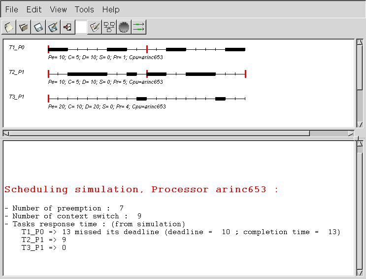
start_section:     partition_duration :  array (tasks_range) of integer;     dynamic_priority :  array (tasks_range) of integer;     number_of_partition : integer :=2;     current_partition : integer :=0;     time_partition : integer :=0;     i : integer;     partition_duration(0):=2;     partition_duration(1):=4;     time_partition:=partition_duration(current_partition); end section; priority_section:     if time_partition=0         then  current_partition:=(current_partition+1)            mod number_of_partition;               time_partition:=partition_duration(current_partition);     end if;     for i in tasks_range loop         if tasks.task_partition(i)=current_partition                   then dynamic_priority(i]:=priority(i);                               else  dynamic_priority(i):=0; tasks.ready(i):=false;         end if;      end loop;     time_partition:=time_partition-1; end section; election_section:         return max_to_index(dynamic_priority); end section;

Figure 5.9 Processes and partitions scheduling into an ARINC 653 system


In this code, tasks.task_partition is a User's defined task parameter. tasks.task_partition stores the partition number hosting the associated task. The variable partition_duration stores the partition cyclic activation table.

VI.2 Scheduling with specific task models.

In the same way you can define specific schedulers, you can also define specific task activation patterns. By default, 3 kinds of task activation pattern are defined in Cheddar :

• Periodic task : a fixed amount of time exists between two successive task activations.
• Aperiodic task : the task is activated only once at a given time.
• Poisson process task : tasks are activated several times and the delay between two successive activations is a random delay. The static variable period in this case is the average time between two successive activations. The delay between activations is generetad according to a random poisson process.

If the application you want to study can not be modeled with this 3 kinds of activation rules above, a possible solution is to explain your own task activation pattern with a user-defined scheduler. The description of task activation pattern is done in .sc files in a particulary section which is called task_activation_section. In this section, you can define named activation rules with set statements. The set statement just link a name/identifier (the left part ot the set statement) and an expression (the right part of the set statement). The expression explains the amount of time the scheduling simulator engine has to wait between two activations of a given task.

start_section: gen1 : random; gen2 : random; exponential(gen1, 200); uniform(gen2, 0, 100); end section; election_section: return max_to_index(tasks.priority); end section; task_activation_section: set activation_rule1 10; set activation_rule2 2*tasks.capacity; set activation_rule3 gen1*20; set activation_rule4 gen2; end section;

Figure 5.10 Defining new task activation patterns : how to run simulation with specific task models

The example of the Figure 5.10 describes a Highest Priority First scheduler which hosts tasks activated with different patterns. Each pattern is described by a set statement :

• The pattern activation_rule1 describes periodic tasks with a period equal to 10.
• The pattern activation_rule2 describes periodic tasks with a period equal to twice their capacity.
• The pattern activation_rule3 describes randomly activated tasks. Two successive activations are delayed by an amount of time which is randomly computed. Delays are computed according to a random exponential distribution pattern with a mean value of 400. 400 is then the average period value of the tasks. The seed used during random delay generation depends on the scheduling options set at simulation time (see section I.3 ) : the user can choose to associate a seed per task or a seed for all the tasks. Seeds can be initialized in a predictable way or in an unpredictable way. In the case of a predictable seed, the random generator is initialized with the seed value given at task definition time or in the scheduling option window. In the case of an unpredictable seed, the seed is initialized by the "gettimeofday" at simulation time.
• The pattern activation_rule4 describes randomly activated tasks. Two successive activations are delayed by an amount of time that is randomly computed. Delays are computed according to a random uniform distribution pattern with a mean value of 50. At each periodic task activation, the period can have a value between 0 and 100. The seed used during random delay generation is managed in the same way than activation_rule3.

When task activation rules are defined, task activation names (ex : activation_rule1) have to be associated with "real" task. The picture below shows you an "Edit/Update tasks" window :

Figure 5.11 Assigning activation rules to tasks

In this example (see the XML project file project_examples/test_user-defined6.xml), the task activation rule activation_rule1 is associated with task T1. The task activation rule activation_rule2 is associated with task T2. The task activation rule activation_rule3 is associated with tasks T3, T4 and T5. Finally, the task activation rule activation_rule4 is associated with tasks T6, T7 and T8. Then, a possible resulting scheduling can be :

Figure 5.12 Scheduling tasks with user-defined task activation pattern

VI.3 Running a simulation with a user-defined scheduler.

Let's see how to run a simulation with one or several user-defined schedulers. First, you have to add a scheduler by selecting the submenu "Edit/Update processors". The following window is then launched :

Figure 5.13 Define a processor with a user-defined scheduler

To add a user-defined scheduler into a Cheddar project, select the right item of the Combo Box and give a name to your scheduler. You should then provide the code of your user-defined scheduler. This operation can be done by pushing the "Read" button.
In this case, the following window is spawned and you should give a file name containing the code of your user-defined scheduler :

Figure 5.14 Selecting the .sc file which contains the user-defined scheduler

By convention, files that contain user-defined scheduler code should be prefixed by .sc. For example, the file rm.sc in our example should almost contain an election section and of course, can also contain a start and a priority sections. When a processor is defined, you have to add tasks on it. To do so, select the submenu "Edit/Update tasks" like in section I. Just place the task on the previously defined processor. Finally, you can run scheduling simulations as the usual case.

Since a user-defined scheduler is also a piece of code, you sometimes need to debug it. To do so, you can use the following tips :

• First, a special instruction can be used to display the value of a variable on the screen : the put statement. For instance, running the following user-defined code will display the value of the dynamic variable to_run each time the scheduler is called :

  --!TRACE start_section: to_run : integer; current_priority : integer; end section; priority_section: current_priority:=0; for i in tasks_range loop  if  (tasks.ready(i)=true) and (tasks.priority(i)>current_priority)             then to_run:=i;                      put(to_run);                  current_priority:=tasks.priority(i); end if; end loop; end section; election_section: return to_run; end section;

  Figure 5.15 Using the put statement
  
• A second tip can help you to test if the syntax of your user-defined scheduler is correct. In all .sc file, you can add the line --!TRACE anywhere. If you add this line, the parser will give extra information during the syntax analysis of your user-defined scheduler. It's useful if you want to test a .sc file before using it in a Cheddar project file. You can also test it with sc, a program designed to read, parse and check .sc files.

VI.4 Looking for user-defined properties during a scheduling simulation.

start_section: i : integer; nb_T2 : integer; nb_T1 : integer; bound_on_jitter : integer; max_delay : integer; min_delay : integer; tmp : integer; T1_end_time : array (time_units_range) of integer; T2_end_time : array (time_units_range) of integer; min_delay:=integer'last; max_delay:=integer'first; i:=0; nb_T1:=0; nb_T2:=0; end section; gather_event_analyzer_section: if (events.type = "end_of_task_capacity") then if (events.task_name = "T1") then T1_end_time(nb_T1):=events.time; nb_T1:=nb_T1+1; end if; if (events.task_name = "T2") then T2_end_time(nb_T2):=events.time; nb_T2:=nb_T2+1; end if; end if; end section; display_event_analyzer_section: while (i < nb_T1) and (i < nb_T2) loop tmp:=abs(T1_end_time(i)-T2_end_time(i)); min_delay:=min(tmp, min_delay); max_delay:=max(tmp, max_delay); i:=i+1; end loop; bound_on_jitter:=abs(max_delay-min_delay); put(min_delay); put(max_delay); put(bound_on_jitter); end section;

Figure 5.16 Example of user-defined event analyzer : computing task termination jitter bound



In the same way that users can define new schedulers, Cheddar makes it possible to create user-defined event analyzers. These event analyzers are also writen with an Ada-like language and interpreted at simulation time.

The event table produced by the simulator records events related to task execution and related to objects that tasks access. Event examples stored in this table can be :

• Events produced when a task becomes ready to run (event task_activation), when a task starts or ends running its capacity (events start_of_task_capacity and end_of_task_capacity),
• Events produced when a task reads or writes data from/to a buffer (events write_to_buffer and read_from_buffer),
• Events produced when a task sends or receives a message (events send_message and receive_message),
• Events produced when a task starts waiting for a busy resource (event wait_for_a_resource), allocates or releases a given resource (events allocate_resource and release_resource).

Each of these events is stored with the time it occurs and with information related to the event itself (eg. name of the resource, of the buffer, of the message, of the task ...). The event table is scanned sequentially by event analyzers. User-defined event analyzers are composed of several sections : a start section, a data gathering section and an analyze and display section.

• As user-defined schedulers, the start section is devoted to variable declarations and initializations.
• The gathering section contains code which is called for each item of the event table. Most of the time, this section contains statements which extract useful data from the event table, and store them for the event analyzer.
• Finally, the display section performs analysis on data previously saved by the gathering section and displays the results in the main window of the Cheddar Editor.

Figure 5.16 gives an example of user-defined event analyzer. From an ARINC 653 scheduling this event analyzer computes the minimum, the maximum and the jitter on the delay between end times of two tasks owned by different partitions (tasks T1_P0 and T2_P1 ; see Figure 5.9).

VI.5 List of predefined variables and available statements.

The tables below list all predefined variables that are available when you write a user-defined code:

Name	Type	Is updated by the simulator engine	Can be changed by user code	Meaning
Variables related to processors
nb_processors	integer	no	no	Gives the number of processors of the current analyzed system.
Variables related to tasks
tasks.period	array (tasks_range) of integer	yes	yes	Stores the value of the parameter given at task definition time. For the meaning of this variable, see section I.
tasks.name	array (tasks_range) of string	no	no	Name of the task
tasks.type	array (tasks_range) of string	no	no	Type of the task (periodic, aperiodic, sporadic, poisson_process or userd_defined)
tasks.processor_name	array (tasks_range) of string	no	no	Stores the processor name of the cpu hosting the corresponding task.
tasks.blocking_time	array (tasks_range) of integer	no	yes	Stores the sum of the bounded times the task has to wait on shared resource accesses.
tasks.deadline	array (tasks_range) of integer	yes	yes	Stores the value of the parameter given at task definition time. For the meaning of this variable, see section I.
tasks.capacity	array (tasks_range) of integer	yes	yes	Stores the value of the parameter given at task definition time. For the meaning of this variable, see section I.
tasks.start_time	array (tasks_range) of integer	yes	yes	Stores the value of the parameter given at task definition time. For the meaning of this variable, see section I.
tasks.used_cpu	array (tasks_range) of integer	yes	no	Stores the amount of processor time wasted by the associated task.
tasks.activation_number	array (tasks_range) of integer	yes	no	Stores the activation number of the associated task. Of course, using this variable is meaningless for aperiodic tasks.
tasks.jitter	array (tasks_range) of integer	yes	yes	Stores the value of the parameter given at task definition time. For the meaning of this variable, see section I.
tasks.priority	array (tasks_range) of integer	yes	yes	Stores the value of the parameter given at task definition time. For the meaning of this variable, see section I.
tasks.used_capacity	array (tasks_range) of integer	yes	no	This variable stores the umount of time unit the task had consumed since its last activation. When tasks.used_capacity reaches tasks.capacity, the task stops to run and waits its next activation
tasks.rest_of_capacity	array (tasks_range) of integer	yes	no	For each task activation, this variable is initialized to the task capacity each time the task starts a new activation. If rest_of_capacity is equal to zero, the task has over its its current activation and then task is blocked upto its next activation.
tasks.suspended	array (tasks_range) of integer	yes	yes	This variable can be used by scheduler programmers to block a task : remove a task from schedulable tasks.
nb_tasks	integer	no	no	Gives the number of tasks of the current analyzed system.
tasks.ready	array (tasks_range) of boolean	yes	no	Stores the state of the task : this boolean is true if the task is ready ; it means the task has a capacity to run, does not wait for a shared resource, does not wait for a delay, does not wait for a offset constraint and does not wait for a precedency constraint.
Variables related to messages
nb_messages	integer	no	no	Gives the number of messages of the current analyzed system.
messages.name	array (messages_range) of string	no	no	Gives the names of each message.
messages.jitter	array (messages_range) of integer	no	no	Jitter on the time the periodic message becomes ready to be sent.
messages.period	array (messages_range) of integer	no	no	Gives the sending period if the message is a periodic one.
messages.delay	array (messages_range) of integer	no	no	time needed by a message to go from the sendrer to the receiver node.
messages.deadline	array (messages_range) of integer	no	no	Stores the deadline if the message has to meet one.
messages.size	array (messages_range) of integer	no	no	Stores the size of the message.
messages.users.time	array (messages_range) of integer	no	no	Stores the time when the task should send or receive the message.
messages.users.task_name	array (messages_range) of string	no	no	Stores the task name that sends/receives the message.
messages.users.type	array (messages_range) of string	no	no	Stores sender if the corresponding task sends the message or stores receiver if the task receives it.
Variables related to buffers
nb_buffers	integer	no	no	Gives the number of buffers of the current analyzed system.
buffers.max_size	array (buffers_range) of integer	no	no	The maximum size of a given buffer.
buffers.processor_name	array (buffers_range) of string	no	no	Gives the processor name that owns the buffer.
buffers.name	array (buffers_range) of string	no	no	Unique name of the buffer.
buffers.users.time	array (buffers_range) of integer	no	no	Stores the time a given task consumes/produces a message from/into a buffer.
buffers.users.size	array (buffers_range) of integer	no	no	Stores the size of the message produced/consumed into/from a buffer by a given task.
buffers.users.task_name	array (buffers_range) of string	no	no	Stores the task name that procudes/consumes messages into/from a given buffer.
buffers.users.type	array (buffers_range) of string	no	no	Stores consumer if the corresponding task consumes messages from the buffer or stores producer if the task produces messages.
Variables related to shared resources
nb_resources	integer	no	no	Gives the number of shared resources of the current analyzed system.
resources.initial_state	array (resources_range) of integer	no	no	Stores the state of the resource when the simulation is started. If this integer is equal of less than zero, the first allocation request will block the requesting task.
resources.current_state	array (resources_range) of integer	no	no	Stores the current state of the resource. If this integer is equal of less than zero, the first allocation request will block the requesting task. After an allocation of the resource, this counter is decremented. After the task has released the resource, this counter is incremented.
resources.processor_name	array (resources_range) of string	no	no	Stores the name of the processors hosting the shared resource.
resources.protocol	array (resources_range) of string	no	no	Contains the protocol name used to manage the resource allocation request. Could be either no_protocol, priority_ceiling_protocol or priority_inheritance_protocol
resources.name	array (resources_range) of integer	no	no	Unique name of the shared resource
resources.users.task_name	array (resources_range) of string	no	no	Gives the name of a task that can access the shared resource.
resources.users.start_time	array (resources_range) of integer	no	no	Gives the time the task starts accessing the shared resource during its capacity.
resources.users.end_time	array (resources_range) of integer	no	no	Gives the time the task ends accessing the shared resource during its capacity.
Variables related to the scheduling simulation
previously_elected	integer	yes	no	At the time the user-defined scheduler runs, this variable stores the TCB index of the task elected at the previous simulation time
simulation_time	integer	yes	no	Stores the current simulation time .
Variables related to the event table
events.type	string	no	no	Type of event on the current index table. Can be task_activation, running_task, write_to_buffer, read_from_buffer, send_message, receive_message, start_of_task_capacity, end_of_task_capacity, allocate_resource, release_resource, wait_for_resource.
events.time	integer	no	no	The time when the event occurs.
events.processor_name	string	no	no	The processor name hosting the task/resource/buffer related to the current event.
events.task_name	string	no	no	The task name related to the current event.
events.message_name	string	no	no	The message name related to the current event.
events.buffer_name	string	no	no	The buffer name related to the current event.
events.resource_name	string	no	no	The resource name related to the current event.

The BNF syntax of a .sc file is given below :

entry := start_rule priority_rule election_rule task_activation_rule gather_event_analyzer display_event_analyzer declare_rule := "start_section:" statements priority_rule := "priority_section:" statements election_rule := "election_section:" statements task_activation_rule := "task_activation_section" statements gather_event_analyzer := "gather_event_analyzer_section" statements display_event_analyzer:= "display_event_analyzer_section" statements statements := statement {statement} statement :=      "put" "(" identifier [, integer] [, integer]")" ";"      | identifier ":" data_type [ ":=" expression ] ";"      | identifier ":=" expression ";"      | "if" expression "then" statements [ "else" statements ] "end" "if" ";"      | "return" expr ";"      | "for" identifier "in" ranges "loop" statements "end" "loop" ";"      | "while" expression "loop" statements "end" "loop" ";"      | "set" identifier expression ";"      | "uniform" "(" identifier "," expression "," expression ")" ";"      | "exponential" "(" identifier "," expression ")" ";" data_type := scalar_data_type      | "array" "(" ranges ")" "of" scalar_data_type ranges := "tasks_range" | "buffers_range" | "messages_range" | "resources_range" | "processors_range" | "time_units_range" scalar_data_type := "double" | "integer" | "boolean" | "string" | "random" operator := "and" | "or" | "mod" | "<" | ">" | "<=" | ">=" | "/=" | "=" | "+" | "/" | "-" | "*" | "**" expression := expression operator expression      | "(" expression ")"      | "not" expression      | "-" expression      | "max_to_index" "(" expression ")"      | "min_to_index" "(" expression ")"      | "max" "(" expression "," expression ")"      | "min" "(" expression "," expression ")"      | "lcm" "(" expression "," expression ")"      | "abs" "(" expression ")"      | identifier "[" expression "]"      | identifier      | integer_value      | double_value      | boolean_value

Notes on the BNF of .sc file syntax :

• entry is the entry point of the grammar.
• The data_type rule describes all data types available in a .sc file
• The operator rule lists all binary operators.
• The expression rule gives all possible expressions that you can use to define your scheduler.
• The statement rule contains all statements that can be used in a .sc file.
• identifier is a string constant.
• integer_value is a integer constant.
• double_value is a double constant.
• boolean_value is a boolean constant.

Two kinds of statements exist to build your user-defined scheduler : low-level and high-level statements. high-level statements operate on all task information. low-level statements operate only on one information of a task at a time. all these statements work as follows :

1. The if statement : works like in Ada or most of programming languages : run the else or the then statement branch according to the value of the if expression.
2. The while statement : works like in Ada or most of programming languages : run the statements enclosed in the loop/end loop block until the while condition becomes false.
3. The for statement : it's an Ada loop with a predefined iterator index. With a for statement, the statements enclosed in the loop are run for each task defined in the TCB table. At each iteration, the variable defined in the for statement is incremented. Then, in the case of task loop for instance (use keyword tasks_range in this case), its value ranges from 1 to nb_tasks (nb_tasks is a predefined static variable initiliazed to the number of tasks hosted by the currently analyzed processor).
4. The return statement. You can use a return statement in two cases :
1. With any argument in any section except in the election_section. In this case, the return statement just end the code of the section.
2. With a integer argument and only in the election_section . Then, the return statement give the task number to be run.
5. The put(p,a,b) statement : displays the value of the variable p on the screen. This statement is useful to debug your user-defined scheduler. If a and b are not equal to zero and if p is an array type, put(p,a,b) displays entries of the table with index between a and b. If a and b are equal to zero and if p is an array, all entries of the array are displayed.
6. The exponential(a,b) statement : intializes the random generator a to generate exponential random values with an average value of b.
7. The uniform(a,b,c) statement : intializes the random generator a to generate uniformly random values between b and c.
8. The set statement : description of new task activation model : assign an expression which shows how to compute task wake up time with an identifier.

The predefined operators work as follows :

1. abs(a) : returns the unsigned value of a.
2. lcm(a,b) : returns the last common multiplier of a and b.
3. max(a,b) : returns the maximum value between a and b.
4. min(a,b) : returns the minimum value between a and b.
5. max_to_index (v) : firstly finds the task in the TCB with the maximum value of v ,and then returns its position in the TCB table. Only ready tasks are considered by this operator.
6. min_to_index(v) : firstly finds the task in the TCB with the minimum value of v, and then returns its position in the TCB table Only ready tasks are considered by this operator.
   
7. a mod b : computes the modulo of a on b (rest of the integer division).

VII. Summary of Cheddar's editor menus and sub-menus

All Cheddar analysis tools are called from the "Tools" menu. This section gives a short description of them. Some of them compute
tasks parameters, and then are composed of two submenus : "Compute and update tasks set"
and "Compute and display".

Choose "Compute and update tasks set" submenu if you want to save computed parameters into your project tasks set.
Choose "Compute and display" if you only want to display computed parameters on the bottom of the main Cheddar window.

Menus and Sub-menus of the Cheddar's editor :

1. File Menu :
   1. New sub-menu : creates a new XML project.
   2. Open sub-menu : loads a XML project file into the editor.
   3. Save sub-menu : saves the current XML project into a file with the current XML project file name.
   4. Save as sub-menu : saves the current XML project into a file with a new XML project file name.
   5. AADL sub-menu : provides ane features related to AADL specifications.
      1. AADL import : reads an AADL specification into Cheddar.
      2. AADL export : translates a Cheddar specification towards an AADL specification.
      3. Export property sets used by Cheddar : writes the Cheddar's property sets into files of the current directory.
      4. Export standard AADL property set : writes the standard AADL property set into files of the current directory.
      5. Customize how AADL services work : allows the user to set some options related to the AADL services provided by Cheddar.
   6. Exit sub-menu : Quit the Cheddar's editor.
   
   
   
2. Edit menu : creates/updates/deletes entities of the current architecture to analyse (entities of the current XML project). Entities can be a processor, a task, a message, a buffer, a network or an event analyzer.
   
   
3. Tools menu :
   1. Clear work space sub-menu : cleans the working area (main window). Does not change anything on the project itself.
      
   
   
   2. Scheduling sub-menu :
      1. Customized scheduling simulation sub-menu : computes and draws scheduling simulation. This sub-menu allows the user to customize the way the scheduling is computed.
      2. Customized scheduling feasibility sub-menu : computes some basics feasibility tests on all processors. The feasibility tests computed there are the utilization factor test and the response time test.
      3. Set priorities according to Rate Monotonic sub-menu : change the task priority according to its period (Tasks with the smallest period become tasks with the highest priority).
      4. Set priorities according to Deadline Monotonic sub-menu : changes the task priority according to its deadline (Tasks with the smallest deadline become tasks with the highest priority).
      5. Partition sub-menu : provides some services to assign tasks on a set of processors.
         1. With Best Fit sub-sub-menu : assigns tasks on the set of processors according to the Best Fit algorithm.
         2. With General Task sub-sub-menu : assigns tasks on the set of processors according to the General Task algorithm.
         3. With Next Fit sub-sub-menu : assigns tasks on the set of processors according to the Next Fit algorithm.
         4. With First Fit sub-sub-menu : assigns tasks on the set of processors according to the First Fit algorithm.
         5. With Small Task sub-sub-menu : assigns tasks on the set of processors according to the Small Task algorithm.
      6. Event table services sub-menu : provides some basic services on event tables.
         1. Compute scheduling and generate event table sub-sub-menu :computes the scheduling and produces the event table.
         2. Draw time line from event table sub-sub-menu : draws time line from the last computed or loaded scheduling/event table.
         3. Run analysis on event table sub-sub-menu : performs analysis on the last computed or loaded scheduling/event table.
         4. Export event table sub-sub-menu : saves the last scheduling/event table into a file with a XML format.
      7. Options sub-menu : describes how the scheduling simulation will be carried out.
      
      
   3. Resource sub-menu :
      1. Bound on blocking time sub-sub-menu : computes bound on shared resources blocking time according to PCP and PIP protocols without computing the scheduling
      2. Looking for priority inversion from simulation sub-sub-menu : runs analysis on a previously computed scheduling to look for high priority tasks blocked by lower priority task at shared resource access.
      3. Looking for priority inversion from simulation sub-sub-menu : runs analysis on a previously computed scheduling to look for tasks blocked forever on shared resources.
      
      
   4. Buffer sub-menu : this submenu can help you to study buffers shared by tasks.
      1. Buffer simulation sub-sub-menu : computes buffer utilization factor and message waiting time from a given scheduling simulation.
      2. Buffer feasibility tests sub-sub-menu : computes bound on buffer utilization factor and message waiting time without computing scheduling.
      
      
   5. Precedency sub-menu : . You will find here some heuristics/algorithms that can schedule or check feasibility of a tasks set with dependencies.
      1. Chetto/Blazewicz modifications on priorities sub-sub-menu : This service creates an independent task set from a dependent task set by modifying task priorities according to precedency constraints.
      2. Chetto/Blazewicz modifications on deadlines sub-sub-menu : This service creates an independent task set from a dependent task set by modifying task deadlines according to precedency constraints.
      3. End to End response time : computes response time from a set of task (which have precendency relationships) with the Holistic method.
      
      
   6. Random sub-menu : this submenu should provide necessary tools to carry out simulations with random events.
      1. Compute response time density sub-menu : compute statistic distribution of task response time from a scheduling simulation.
      
      
      
4. Help Menu :
   1. About Cheddar sub-menu : provides version number of the Cheddar's binaries.
   2. Manual sub-menu : contains the text given in this section.
   3. Scheduling references sub-menu : gives all paper references used to compute feasibility tests and simulation results.

Contact : Frank Singhoff mailto:singhoff@univ-brest.fr
Last update : December the 4th, 2008