Real-time scheduling analysis of SDF graphs: an example with Cheddar
Hai Nam Tran (hai-nam.tran@univ-brest.fr), Frank Singhoff (singhoff@univ-brest.fr)
Summer school "Adaptive Machine Learning at the Edge (AMLE)", Lorient, 13-16 June, 2022
Table of contents
Introduction
The objective of this lab is to experiment several classical algorithms and analysis methods of the real-time scheduling theory.
For such a purpose, we will use Cheddar.
- Part I shows how to model a software architecture and how to analyse it.
- Part II presents and compare classical real-time scheduling algorithms.
- Part III addresses shared resources.
- Part IV proposes full software architectures to be modeled and verified.
Ideas of the exercises in this tutorial were taken from [COT 00, BUR 97, DEM 99, KRI 97].
We can look for those books for extra exercises.
-
Cheddar was installed on the PCs used for this tutorial. You can open the Cheddar folder found in
~/bin/Cheddar-3.3-Linux64-bin
- The other distributions of Cheddar is also available to download here.
Instruction to install Cheddar can be found in the file
HOWTO_INSTALL.txt
-
In a terminal, navigate to the Cheddar folder (
$ cd ~/bin/Cheddar-3.3-Linux64-bin) and run Cheddar ($ ./cheddar)
-
The window of the Figure 1 should be displayed:
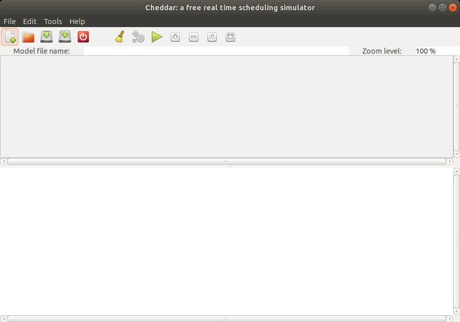 Fig. 1: Main window of Cheddar
-
The top part of this window (in gray in the figure) displays the time lines computed during scheduling simulation.
The bottom part of this window displays numeric analysis results.
In this section, we will design our first Cheddar model.
Let describe the architecture of the real-time system we want to verify.
For such a purpose, we will use the Cheddar built-in ADL
(ADL stands for Architecture Description Language), called Cheddar ADL.
Cheddar ADL is an architecture description language dedicated to real-time scheduling analysis.
A Cheddar ADL model is composed of a description of both the hardware and of the software part of the system to analyse.
Those models can be written with any editors, but in the sequel, we will use the graphical editor of Cheddar as follow:
-
First, the hardware components composing the execution environment running the software must be descrided.
With Cheddar, the execution platform can be composed of one or several
processor components embedding each one or several
core components with optionnal cache components.
A core component models a unit of computation, i.e. an entity providing the support to run one or several tasks.
-
To describe a
core component, use the menu Edit/Hardware/Core which opens the windows of the Figure 2:
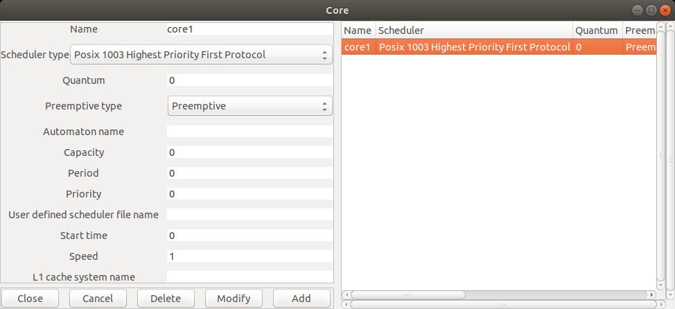 Fig. 2: Editing a core
-
A
core component is defined by the following attributes:
-
Name: the unique name of the component, here, core1.
-
Scheduler type: the way tasks will be allowed to share the core,
i.e. the scheduling policy
assigned to the core.
In the window above, the core component owns a preemptive fixed priority scheduler compliant with POSIX 1003
(value POSIX_1003_Highest_Priority_First_Protocol for the Scheduler type attribute).
In Cheddar, with such scheduler, allowed priority values ranges from 0 to 255
(255 is the highiest priority level).
As with Linux, priority 1 to 255 are devoted to SCHED_RR and SCHED_FIFO tasks
while
priority level 0 is devoted to the SCHED_OTHER policy.
Such policies allow Cheddar to compute a deterministic scheduling even when the software architecture
model have several tasks with equal priorities.
-
Preemptive type: specicy if the scheduler is preemptive or not.
- The other attributes can be ignored for such tutorial.
All the window you may use to edit Cheddar ADL components have the same interface:
-
Button
Add: allows you to add a component to the architecture model.
-
Button
Delete: allows you to delete a component from the architecture model.
Before pushing this button, you must select the targetted component in the component list in the right side of the window.
-
Button
Modify: this button has a behavior similar to the Delete button, excepts that the
component is updated with the values of the attributes in the left part of the window.
-
Button
Close: closes the window and validates all the updates made since the windows was opened.
-
Button
Cancel: closes the window and cancels all the updates made since the windows was opened.
-
Once
core1 is defined, we can define processor components that
use
core1 with the
Edit/Hardware/Processor menu, which displays the following windows:
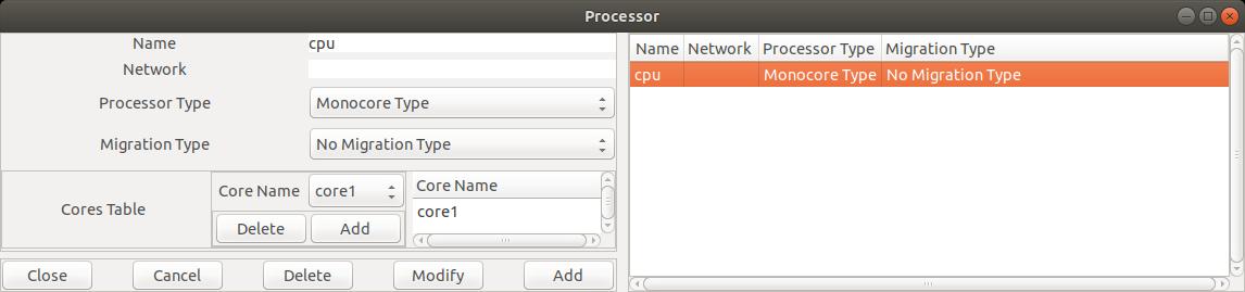 Fig. 3: Editing a processor component
In the Figure 3, we define a processor named
Fig. 3: Editing a processor component
In the Figure 3, we define a processor named cpu1 which is composed of the core1
component.
Adding or deleting a core inside a processor can be achieved with the buttons
Add and Delete from the subwindows called Cores Table.
In this lab, we restrict ourself with uniprocessor architecture models. Then,
processor only contains
one core component and then, we need to set Processor Type and Migration Type
attributes
respectively to
Monocore Type and
No Migration Type values.
-
In the sequel, we express the software part of the system to analyse.
For this lab,
this software part is mainly composed of the tasks and the shared resource components.
(
task Cheddar ADL component type and
resource component type).
Other software components exist in Cheddar ADL, but they are not required there (See the
Cheddar ADL reference guide for further details).
task and
resource components have to be defined inside
Address Space components.
An Address Space component can be seen as a entity modelling
the concept of
an application, or a Unix process address space, or even an ARINC 653 partition.
-
The window of the Figure 4
(menu
Edit/Software/Address space)
shows you how to define an
Address Space for this tutorial.
The only attributes we have to define are
Name and Cpu Name.
For the next exercises, we have to define one
Address Space component for each processor component.
However, for specific analysis as ARINC 653 or more generally,
hierarchical architecture models,
more attributes have to be specified for such kind of component.
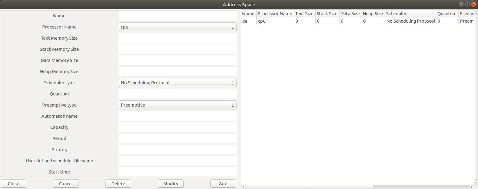 Fig. 4: Editing an address space component
-
The last step, to edit a Cheddar ADL model, is to specify task parameters, which can
be achieved with the menu
Edit/Software/Task:
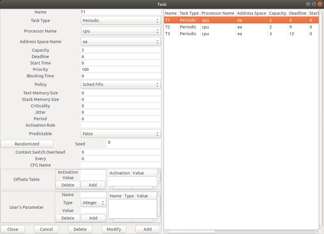 Fig. 5: Editing a task component
Again, such component type have mumerous attributes. The most importants are:
Fig. 5: Editing a task component
Again, such component type have mumerous attributes. The most importants are:
-
Name: the unique name of the component.
-
Task type: the type of the task, which specifies how the task will be released.
A task may be periodic, sporadic, released according to a poisson process (e.g. poisson task type),
GMF, aperiodic, ...
-
Capacity: the WCET of the task.
-
Period: the delay between two successive release times of the task.
-
Deadline: the deadline the task has to meet. It is a delay relative to the period of the task (i.e. not an absolute deadline).
-
Address space name and CPU name where the task is supposed to be located/run.
-
Priority: priority level assigned to the task. 255 is the higher level of priority; 0 is the lower.
In the example of the Figure 5, we have defined 3 tasks, which were periodic, synchronous, with deadlines on
requests, and then, which were defined with the following attributes:
- Task T1:
Capacity = 2, Deadline = 6, Period = 6
- Task T2:
Capacity = 2, Deadline = 9, Period = 9
- Task T3:
Capacity = 3, Deadline = 12, Period = 12
-
Priority attributes were assigned according to Rate Monotonic within the allowed priority range (from 1 to 255).
- You should notice that the deadlines are equal to the periods (see attribute
Deadline).
- Finally, the attribute
Start time is set to 0 in order to model a synchronous task set.
Cheddar provides features to load/save a model in the Cheddar ADL format.
-
File/Save XML Project: a system modeled in Cheddar can be exported in a XML file respecting the Cheddar ADL format.
-
File/Open XML Project: a model can be imported to Cheddar to be analyzed.
In this tutorial, for several exercises, the models are available to download.
In this last section, we show how to perform an analysis of the architecture model previously designed.
From the menu Tools and for a given
architecture model, we can perform 3 types of analysis with Cheddar:
-
We can use simulation tools to compute
the scheduling of a task set, and then, from such scheduling,
to compute various performance criteria (worst/average/best response times, missed deadlines, blocking time
on shared resources, deadlocks, ...).
-
We can also call various feasibility tests that allow
the designers to check deadlines without computing
the scheduling of the task set.
-
If the previous tools have shown that some deadlines cannot be met, we can also
improve the architecture
model by various means: priority assignments, task partitionning, task clustering,
...
Under the menu, some buttons allow you to quickly access to a summary of those Cheddar analysis features
(all analysis features can be accessed by the Tools menu).
Indeed, the  button starts a scheduling simulation and the
 button computes a sample of
feasibility tests for a basic periodic task set.
Basically, the button computes
worst case task response time following the
Joseph et Pandia [JOS 86] method extended for any Deadline and classical CPU bound tests.
Again, for specific feasibility tests (e.g. transactions), see the
button computes a sample of
feasibility tests for a basic periodic task set.
Basically, the button computes
worst case task response time following the
Joseph et Pandia [JOS 86] method extended for any Deadline and classical CPU bound tests.
Again, for specific feasibility tests (e.g. transactions), see the Tools menu.
Figures 6 et 7 show a screenshot of Cheddar for the model edited in section
I.2, and for results produced by buttons
and
.
We can see there worst case response times computed by the
Joseph and Pandia [JOS 86] method and also by the scheduling simulation
on the feasibility interval.
Feasibility tests on cpu utilization factor cannot be applied there
as the tool cannot be
sure that priorities have been assigned according to Rate Monotonic. To apply this test, one
must change the
scheduling policy of the core1 component with the Rate_Monotonic_Protocol value.
We can also notice in the time lines that vertical red rectangles show task release times.
Horizontal rectangles
show when tasks are running. Many other display options exist there and can be modified by the
Tools/Scheduling/Scheduling Options menu.
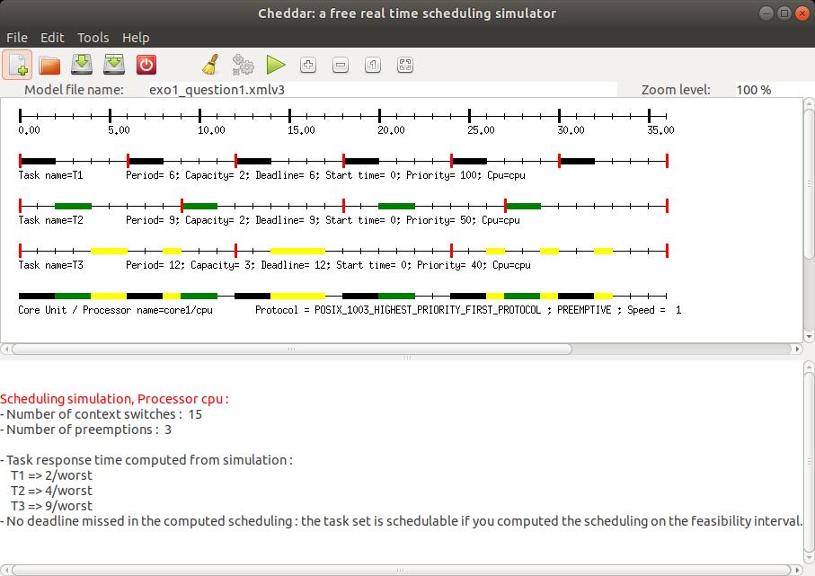 Fig. 6: A scheduling simulation
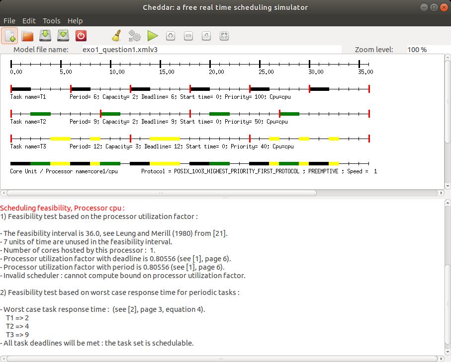 Fig. 7: Compute schedulability feasibility tests
Let see now our first true exercise.
Exercise 1
- Edit a Cheddar model for the system analyzed in the figures 6 and 7, and then, with buttons
and ,
check that you get the results of the figures 6 and 7.
- From the scheduling simulation, read the different response times for each task
(remind that response time = completion time - release time).
For a given task, can you see the response time varying during the scheduling simulation ? Why ?
When should we see the shortest response time ? Why ?
- Update the parameters of the tasks as follows:
- Task T1 :
Capacity = 2, Deadline = Period = 6, Start time = 0
- Task T2 :
Capacity = 8, Deadline = Period = 24, Start time = 0
- Task T3 :
Capacity = 4, Deadline = Period = 12, Start time = 0
- Priority : apply Rate Monotonic.
This task set is said to be harmonic as each period is multiple with the other periods of the task set.
For such a kind of task set, we know that we can meet task deadlines even if the processor is busy
upto 100%, provided a preemptive fixed priority scheduling policy and a Rate Monotonic priority
assignment are applied.
- With Cheddar, compute the scheduling simulation during the feasibility interval (button ).
From this simulation, check the schedulability of this task set.
In this part, we experiment and compare classical scheduling policies.
Exercise 2
We consider two periodic tasks, synchronous and with
deadline on request : tasks T1 and T2.
They are defined as follow:
- Task T1 :
Capacity = 4, Deadline = Period = 8, Start time = 0
- Task T2 :
Capacity = 5, Deadline = Period = 10, Start time = 0
- Priority are assigned according to Rate Monotonic.
- Open the model for this exercice: exo_sched_1_base.xmlv3. It consists of a processor composed of one core.
- Edit this Cheddar model for the task set running on the processor.
- Edit the core to host a preemptive fixed priority scheduler.
- With Cheddar, compute a scheduling simulation for the feasibility interval
(button ).
- From this simulation, what are the worst case response times of each task?
Can we see missed deadlines?
- Change you Cheddar model in order to use a preemptive EDF instead
(value
Earliest_Deadline_First_Protocol for the Scheduler type attribute).
Do again questions 2 and 3.
- Compare both analysis results. What can you see? Is it surprising?
- Change again your model: now we consider a preemptive EDF with the same task sets, but you must
add now an aperiodic task.
We do not require that the deadline of this aperiodic task must be met.
To define such aperiodic task, change
the value for the attribute
Task Type (see. figure 5):
- Periodic task T1:
Period=Deadline=8, Capacity=4, Start time = 0
- Periodic task T2:
Period=Deadline=16, Capacity=8, Start time = 0
- Aperiodic task T3:
Deadline=15, Capacity=4, Start time = 0
- Compute again the scheduling simulation for the first 30th units of time (button ).
What can you see now?
- What can we conclude about the suitability of EDF for critical real-time systems?
Is it the case with fixed priority scheduling?
Exercise 3
We consider a simple SDF graph provided in Figure 8
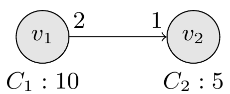 Fig. 8: A simple SDF graph
The two actors are mapped to two periodic tasks as follow:
Fig. 8: A simple SDF graph
The two actors are mapped to two periodic tasks as follow:
- Task T1 :
Capacity = 10, Deadline = Period = 30, Priority = 2, Start time = 0
- Task T2 :
Capacity = 5, Deadline = Period = 15, Priority = 1, Start time = 0 .
- Two tasks are scheduled on one core under the
POSIX_1003_Highest_Priority_First_Protocol scheduler
- Open the Cheddar model exo_sdf_simple_1.xmlv3.
It consists of the two tasks above and a processor.
-
To model the communication between actors in SDF graphs, the
Buffer entity is used in Cheddar.
To add a Buffer, go to Edit > Software > Buffer.
- Buffer 1:
Buffer size = 1, Initial Data Size = 0
- Task T1 produces 2 tokens to the buffer at its 10th unit of execution time
- Task T2 consoumes 2 tokens to the buffer at its 1st unit of execution time
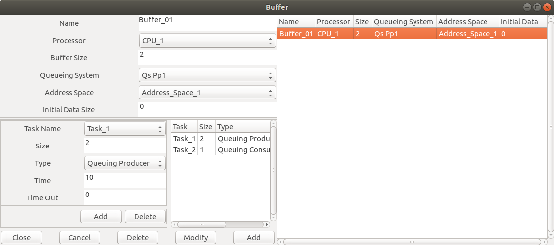 Fig. 10: Editting a buffer component
-
Cheddar also requires us to explicily specifies the dependencies between tasks and buffers.
To do so, go to
Edit > Software > Dependencies > Queueing Buffer and add 2 dependencies.
- 1 dependency between Task T1 and buffer B1, with the orientatation
From Task to Object
- 1 dependency between Task T2 and buffer B1, with the orientatation
From Object to Task
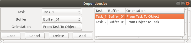 Fig. 11: Editting dependencies
-
Run the simulation, we should obtain the following result:
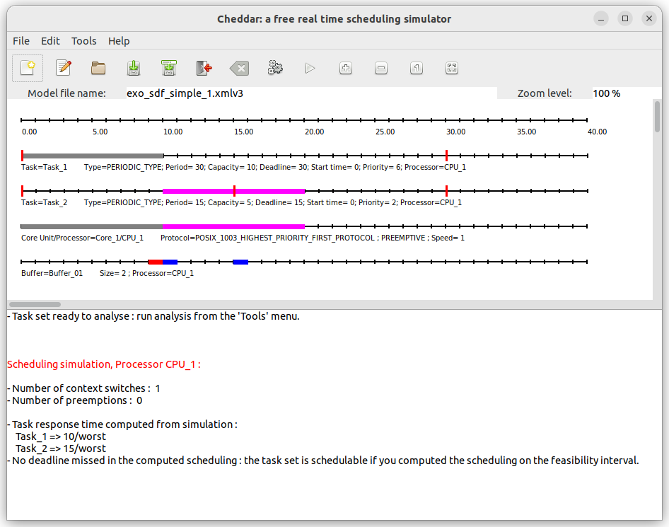 Fig. 11: Simulation with buffers
We use the following color code to describe interactions between tasks and buffers
Fig. 11: Simulation with buffers
We use the following color code to describe interactions between tasks and buffers
- Red - produce to buffer
- Light Red - buffer overflow, not enough spaces to produce tokens
- Blue - consume from buffer
- Light Blue - buffer underflow, not enough tokens to consume
-
What are the problems when the WCET of task T2 becomes 10 ? Suggest a solution by modifying scheduling parameters ?
Exercise 4
We consider the SDF graph provided in Figure 9.
In order to generate FPP scheduling of this graphs, the following elements have to be considered.
- Tasks scheduling parameters (representing the actors): capacities, periods, deadlines, offsets
- Number of processors, buffer sizes, number of initial tokens, max throughput
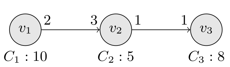 Fig. 9: SDF graph to model
The computation of all these parameters are not straightforward.
As we have seen in the lecture, these parameter can be computed by using tools such as ADFG (presented in the lecture).
- Open the Cheddar model exo_sdf_1.xmlv3.
It consists of two processors, three tasks, two buffers with computed scheduling parameters.
- Analyze and note the scheduling parameters in the model.
- Run scheduling simulation of the model. Is the throughput of the graph maxed ?
- Modify the priorities so that task 3 have a higher one than task 2. What is the problem ?
In the previous exercise, we assumed the tasks as independent.
In the sequel, we illustrate the use of Cheddar with dependent tasks: with tasks
sharing resources according to classical protocols such as PCP or PIP.
Exercise 5
We consider three periodic tasks, synchronous and
with deadlines on request: tasks T1, T2 and T3.
They are defined as follow:
- Task T1:
Period=Deadline=6, Capacity=2, Start time = 0
- Task T2:
Period=Deadline=8, Capacity=2, Start time = 0
- Task T3:
Period=Deadline=12, Capacity=5, Start time = 0
We assume a preemptive fixed priority scheduling policy and we apply Rate Monotonic to assign priorities.
We also assume that tasks T1 and T3 share a resource named S.
T1 and T3 access to S in mutual exclusion:
-
T3 needs S during all its capacity.
-
T1 needs S during the 2nd unit of time of its capacity only.
-
Open the model for this exercice: exo_shared_resource_1_base.xmlv3.
It consists of a processor composed of one core and the task set described above.
-
We edit our Cheddar model for the resource S.
To define S, we need the
Edit/Software/Resource menu which displays the following window:
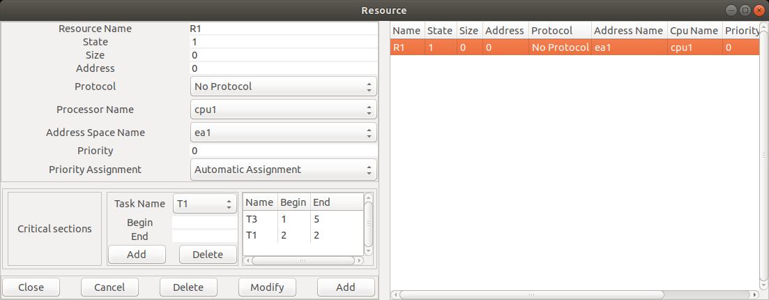 Fig. 8 : editing a resource component
In this window, and for our lab, we need to set the following attributes:
Fig. 8 : editing a resource component
In this window, and for our lab, we need to set the following attributes:
-
Name : the unique name of the shared resource.
-
CPU Name and Address space name: give where the resource is located.
-
State: is the status of the resource.
A Cheddar ADL resource may be seen as a
counting semaphore.
A Cheddar ADL resource has an integer value.
When a task allocates a resource, its counter is
decremented. When a task releases a resource, its counter is incremented.
When this counter is equal or less than 0, a task which requests the resource
is blocked as the resource is already allocated.
For our exercises,
State must be set to 1.
-
Protocol: is the protocol to apply when a resource is handled by a task.
The value No Protocol means that the simulator will apply no priority inheritance and that
the blocked tasks on the semaphore are stored in a FIFO queue.
In this exercise and in the next one, we will alo use the values
Priority Inheritance Protocol (or PIP) and
Priority Ceiling Protocol (or PCP)
when we need to apply inheritance protocols.
Right now, you must set this attribute with the value
No Protocol for the resource S.
-
Priority assignment : specify if the ceiling priority of
the resource component
will be computed automatically by Cheddar, or assigned manually by you.
For our exercises, we have to set this attribute to
Automatic Assignment.
-
Critical sections: in this part, we specify when each task needs the shared resources.
Begin is the start time of each critical section and End
is the critical section completion time.
The buttons Add and Delete allow the designer
to create or remove a critical section for a given resource.
As an example, the Figure 8 shows how to express that T1
needs the resource at the beginning of its 2nd unit of time and
releases the resource at the end of this unit of time.
Again in this Figure, we can see that T3 needs the resource during all its capacity
(i.e. before starting
the 1st unit of time and after its 5th unit of time).
-
Compute the scheduling simulation on the feasibility interval
(button ).
You should get the scheduling simulation of the Figure 9.
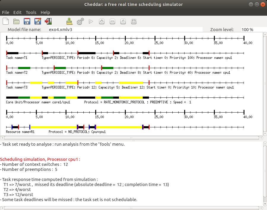 Fig. 9: scheduling simulation with a shared resource
- On the resource time line, horizontal rectangles show when the resource is used.
Those rectangles are colored as the tasks are (see
option in the
Tools/Scheduling/Scheduling Options menu).
Furthermore, bleu vertical rectangles show when the resources are locked while red vertical rectangles show
when resources are unlocked.
-
In this time line, find when tasks T1 and T2 lock and unlock S.
-
From this time line, can we see priority inversions? Where?
-
Change S protocol by
Priority Inheritance Protocol (or PIP), and compute again the scheduling simulation.
With PIP, a task which blocks another with a higher priority, runs its critical section
with the blocked task priority.
-
What can we see in this new scheduling simulation about the shared resource?
-
Say at which time the priorities of the tasks change due to PIP.
-
With the
button, compute the worst case response time with the
Joseph et Pandia method and compare those results with the one computed during the scheduling simulation.
What can you see? Explain.
-
From the scheduling simulation, give the blocking time of each task due to the shared resource S.
Exercise 6
We investigate a system embedded in a car which displays various data to the driver.
This system is composed of several tasks and we expect to verify their timing behavior.
The system is composed of 5 tasks:
- Task SENSOR_1 reads every 10 ms the speed of the car.
- Task SENSOR_2 reads every 10 ms the temperature inside the car.
- Task SENSOR_3 reads every 40 ms the GPS position of the car.
- Task DISPLAY_1 produces on a screen every 12 ms a summary of the data retrieved
by the three sensor tasks.
- Finally, tasks DISPLAY_2 displays on a second screen the map of the current location of the car.
This display is made on request by the driver every 6 ms.
An enginer implements all those tasks and then, run them alone on the targetted system.
After several measurements, he shows that:
- Task SENSOR_2 and DISPLAY_1 execution times never exceed 2 ms.
- Task SENSOR_3 needs between 2 and 4 ms to successfully run its code.
- Finally, tasks SENSOR_1 and DISPLAY_2 have an execution time of less than 1 ms.
We assume that all tasks start their first activation at the same time.
Furthermore, all tasks must complete their current activation before they have to start the next one.
We assume an execution platform composed of one processor which provides a preemptive fixed priority scheduler.
Priorities range from 0 to 31. 0 is the lowest priority value.
The system does not allow designers to assign the same priority value to several tasks.
Question 1:
- Usually, what are the criteria to assign priority to tasks?
- Assign a priority level for each task. Motivate your choices.
Question 2:
With Cheddar, from the priority assignment of the previous question, compute the
worst case response times with the Joseph and Pandia method for the
SENSOR_1, the SENSOR_2, and the SENSOR_3 task.
Question 3:
In fact, tasks
SENSOR_1,
SENSOR_2,
and SENSOR_3
share a memory area protected by a semaphore (i.e. accessed in mutual exclusion).
SENSOR_1 et SENSOR_2 needs this memory during all their capacity
while
SENSOR_3 only needs it during the 2 first units of time of its capacity.
The semaphore protecting the memory applies the PIP protocol.
Explain why the worst case response times computed in the previous question are not true
anymore.
Question 4:
With Cheddar, compute the scheduling of this task set on the 60th first units of time.
Say when the shared resource is allocated and released. Say also if some priority inversions
occur. Finally say when the priorities of the tasks change due to PIP.
Question 5:
For the questions 5 and 6, we now assume that all tasks are independent.
In order to activate more frequently the tasks, we experiment the scheduling of those
tasks on a two processor platforms : processors
a and b.
Migrations of the tasks are not allowed: we then apply a partitionning approach.
The tasks are defined according to those parameters:
- Task DISPLAY_1: Processor = b ;
Capacity = 4, Period=Deadline= 6
- Task SENSOR_1: Processor = b ;
Capacity = 2, Period=Deadline= 20
- Task DISPLAY_2: Processor = a ;
Capacity = 2, Period=Deadline= 3
- Task SENSOR_2: Processor = a ;
Capacity = 2, Period=Deadline= 5
- Task SENSOR_3: Processor = a ;
Capacity = 2, Period=Deadline= 5
The tasks are scheduled according to a preemptive fixed priority scheduling policy.
Task priorities are assigned according to Rate Monotonic.
Show without scheduling simulation that it exists at least one task which cannot meet its deadline.
Question 6:
In fact, tasks were assigned to processors randomly.
All tasks can run on both processors.
Processors
a and
b only differ from their execution speed:
On
processor b, a task runs twice more quickly than on
processor a.
Assign tasks to processors
a and b such as all task deadlines can be met.
Explain your choice.
-
[BUR 97] A. Burns and A. Wellings. Real-time Systems and Programming Languages. Addison Wesley, 1997.
-
[COT 00] F. Cottet, J. Delacroix, C.Kaiser, and Z. Mammeri. Ordonnancement temps réel. Hermès, 2000.
-
[DEM 99] I. Demeure and C. Bonnet. Introduction aux systèmes temps réel. Collection pédagogique de télécommunications, Hermès, Septembre 1999.
-
[JOS 86] M. Joseph and P. Pandya. Finding Response Time in a Real-Time System. Computer Journal, 29(5):390--395, 1986.
-
[KRI 97] C.M. Krishna and K.G. Shin. Real-Time Systems. Mc Graw-Hill International Editions, 1997.