
Many critical systems are organized as an oriented graph of tasks.
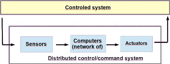
It may be the case of control-command systems as shown in the figure above.
Control-command systems are in charge to manage a system, which is usually a
hardware component. Most of the time, the control-command system observe the behavior
of the hardware controled device with sensors, analyse the current status of the controled
device, and then sends command to adapt its behavoir in order to achieve a given goal.
Commands are sended by the actuators.
The computing part of a control-command system may be complex and sometimes distributed, i.e.
composed of several computing units connected by network devices.
In this kind of computing system, it is also usual to organize the computing software component,
i.e. the tasks running the sensing, the analysis and the actuating programs, as a oriented graph.
In this recipe, we only focus on the flow of data aspect of tasks composing the control-command system.
We assume in this recipe a uniprocessor architecture: distributed aspect is
specifically addressed in recipe 7.
Here is a simplified example of this recipe
(which can be downloaded here):
PACKAGE dataflow_Pkg
PUBLIC

DATA my_data
END my_data;

THREAD a_thread
FEATURES
  input : IN DATA PORT my_data;
  output : OUT DATA PORT my_data;
END a_thread;

PROCESS my_process
FEATURES
  input : IN DATA PORT my_data;
  output : OUT DATA PORT my_data;
END my_process;

PROCESSOR cpu
PROPERTIES
   Scheduling_Protocol=>HPF;
END cpu;

SYSTEM dataflow
END dataflow;

PROCESS IMPLEMENTATION my_process.source_impl
SUBCOMPONENTS
  T1 : THREAD a_thread
    { Dispatch_Protocol => Periodic;
      Compute_Execution_Time => 3 ms .. 3 ms;
      Period => 20 ms;
      Priority => 30;
      Deadline => 20 ms; };
CONNECTIONS
  C0 : PORT input -> T1.input;
  C1 : PORT T1.output -> output;
PROPERTIES
  Timing => immediate applies to C0, C1;
END my_process.source_impl;


PROCESS IMPLEMENTATION my_process.sink_impl
SUBCOMPONENTS
  T2 : THREAD a_thread
    { Dispatch_Protocol => Periodic;
      Compute_Execution_Time => 3 ms .. 3 ms;
      Period => 20 ms;
      Priority => 10;
      Deadline => 20 ms; };
  T3 : THREAD a_thread
    { Dispatch_Protocol => Periodic;
      Compute_Execution_Time => 3 ms .. 3 ms;
      Period => 20 ms;
      Priority => 100;
      Deadline => 20 ms; };
CONNECTIONS
  C0 : PORT input -> T2.input;
  C1 : PORT T2.output -> T3.input;
  C2 : PORT T3.output -> output;
PROPERTIES
  Timing => immediate applies to C0, C1, C2;
END my_process.sink_impl;

SYSTEM IMPLEMENTATION dataflow.impl
SUBCOMPONENTS
  process1 : PROCESS my_process.source_impl;
  process2 : PROCESS my_process.sink_impl;
  my_platform : PROCESSOR cpu;
PROPERTIES
  Actual_Processor_Binding => ( reference(my_platform) ) applies to process1;
  Actual_Processor_Binding => ( reference(my_platform) ) applies to process2;
END dataflow.impl;


END dataflow_Pkg;
The graphical representation of this example is:

In this recipe, threads are organized as a graph to implement a
flow of data. We assume two processes: a source process sending the messages and
a sink process receiving them.
The two processes are located on the same processor/computing units.
The processes could be located on different processor, which leads to possible
communication delays, but it is outside the scope of recipe 3 (see recipe 7 for such purpose).
Threads exchange messages throught data ports.
Communication semantics is defined by the semantics of the data port
category and the Timing property that refines the data port semantics.
The semantics of communications with data ports is:
- Messages are sent at completion time of senders.
- Receivers read messages at their dispatch time.
Timing property may have 3 possible values making reference to 3 different
protocols. These protocols will imply specific behavior of the thread scheduling
and of the data receiving threads may receive.
Those protocols are:
- sampled. With this protocol, the scheduling of threads is not changed
by data port communication. Sending and receiving threads stay independent from a scheduling
perspective. When receiving threads read data, they simply read the last written value.
Notice that if receiving threads have period smaller than sending threads, this
protocol may imply that written data could be never read.
Notice also that if receiving threads have period larger than sending threads, this
protocol may imply that written data could be read several times. In fact, with a
sampling port connection, so semantic on read/written data is enforced.
- immediate. With an immediate data port connection, when a sending thread
emits a message, it dispatchs immediatly the receiving threads. This procolo may reduce
the latency betwenn emission and reception of data. It may also help to not lose messages and
to not read twice the same messages. It's main drawback is that it makes scheduling decisions
and communications decision dependent.
- delayed. With delayed connections, receiver threads are dispatched
later than sending threads. A fixed delay is enforced between the dispatch of the receivers
and the senders. Assuming that both receiving and sending threads have the same period
p, when a sender is dispatched at time k to send its kth message,
receivers will be dispached to read message kth at time k+p.
As there is a delay between message sending and the dispatching of the receiving
threads, delayed connections increase communication latencies, which
With the example of this recipe, we have 3 threads interacting by data ports.
Those threads exchanges messages of type my_data.
All connections of this example are refined with an immediate Timing properties.
This recipe can raise two different analysis:
- As explained at recipe 1, one can
call scheduling analysis to compute Worst Case Response Time of each thread.
In recipe 3, there is no shared data component to analyze, so analysis presented
in recipe 2 are not revelant.
- More specifically with this recipe about flow of data met in
controlled/command systems, one may want to evaluate the
worst case latency from the data read by sensors and the order sent to actuators.
Imagine a car on which the driver push the
brake pedal, what you may want to know is not how much time the controller of the break
pedal read the pressure .... but how many time the controller will take to send
the order to the disc to strart reducing speed of the vehicule.
This latency is said to be an "end to end latency" as several components could be crossed
from the sensor upto the actuator. You can even imagine that between the sensor and the
actators, network devices must be crossed and several applications must be run.
Then verifying that end to end latency is smaller or equal to a given deadline
can be a complex work to do.
Finally, notice that AADL also brings the concepts of flow,
as shown in the following example. The flow concept allows designer to express
explicitly flow of data on which the designer expect verification.
Flow specification starts with thread types in which one may declare that the component
can be part of flow. The main declaration is at the process level: in this example,
the flow is declared to cross threads T1, T2 and T3. A deadline of 1 second assigned
to the process specift the requirement on the worst case end to end latency, which must
be verified as smaller than 1 second.
DATA my_data
END my_data;

THREAD T1
FEATURES
	output: out data port my_data;
FLOWS
	f1: flow source output;
PROPERTIES
	Deadline => 100 ms;
	Dispatch_Protocol => Periodic;
	Period => 1000 ms;
END T1;

THREAD T2
FEATURES
	input: in data port my_data;
	output: out data port my_data;
FLOWS
	f2: flow path input -> output;
PROPERTIES
	Deadline => 50 ms;
	Dispatch_Protocol => Periodic;
	Period => 1000 ms;
END T2;

THREAD T3
FEATURES
	input: in data port my_data;
FLOWS
	f3: flow sink input;
PROPERTIES
	Deadline => 70 ms;
	Dispatch_Protocol => Periodic;
	Period => 1000 ms;
END T3;

PROCESS my_process
END my_process;

PROCESS IMPLEMENTATION my_process.impl
SUBCOMPONENTS
  T1 : THREAD T1;
  T2 : THREAD T2;
  T3 : THREAD T3;
CONNECTIONS
  C0 : PORT T1.output -> T2.input;
  C1 : PORT T2.output -> T3.input;
FLOWS
  flow1: end to end flow
	T1.f1 -> c0 -> T2.f2 -> c1 -> T3.f3;
PROPERTIES
  Timing => immediate applies to C0, C1;
  Deadline => 1000 ms;
END my_process.impl;
From the flow concept, OSATE and
AADLInspector are able to compute such end to end latency. Below is a AADLInspector
model showing end to end latency for an other example for this recipe:
SYSTEM my_system
END my_system;

SYSTEM IMPLEMENTATION my_system.others
SUBCOMPONENTS
  Sensors : SYSTEM Sensors.i;
  Processing : SYSTEM Processing.i;
  Actuators : SYSTEM Actuators.i;
  Communication : BUS CAN;
CONNECTIONS
  mes_cnx : PORT Sensors.measures -> Processing.measures {Timing => Immediate;};
  cmd_cnx : PORT Processing.commands -> Actuators.commands {Timing => Immediate;};
FLOWS
  f1 : END TO END FLOW Sensors.f1 -> mes_cnx -> Processing.f1 -> cmd_cnx -> Actuators.f1;
  f2 : END TO END FLOW Sensors.f2 -> mes_cnx -> Processing.f1 -> cmd_cnx -> Actuators.f1;
PROPERTIES
  Actual_Connection_Binding => ( reference(Communication) ) applies to mes_cnx, cmd_cnx;
ANNEX LAMP {**
  write('=== list of the elements of flow f1:'), nl,
  getEndToEndFlow('root','f1',L), printList(L),
  write('=== latency of all the end to end flows:'), nl,
  getFlowsLatency
**};
END my_system.others;
The end to
end latency includes communications delays from data port connection protocols and
also worst case execution time of the emmiter and receiver threads, that compete
for the processor with the other threads that are not part of the data.
Then AADLinspector first compute thread worst case response before putting this
timing result in the end to end flow analysis.
To actually run the end to end flow analysis, AADLInspector call its LAMP plugin
by the annex subclause:
 ANNEX LAMP {**
  write('=== list of the elements of flow f1:'), nl,
  getEndToEndFlow('root','f1',L), printList(L),
  write('=== latency of all the end to end flows:'), nl,
  getFlowsLatency
**};
which is attached to the root component system. The result of the analysis is shown
in this screenshot, in the right part of the window:
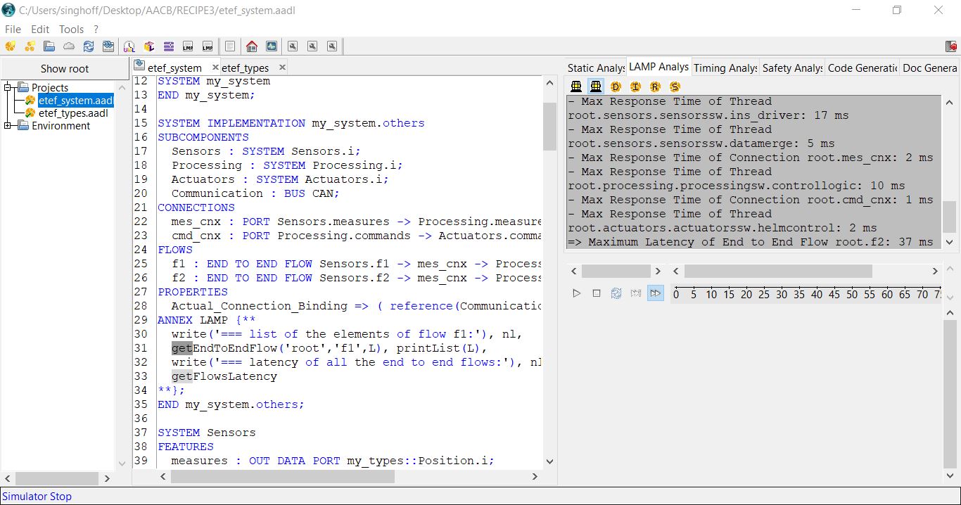
The end to end flow latency is about 23 ms for flow f1 and 37 ms for flow f2.
Notice that worst case response time here are computing with the Marzhin simulator, but
of course it could be computed by any schedulability tools as Cheddar for example.
AADL model files for this example is available here.
A simple case study, as an example
The figure above presents a software architecture
composed of 7 periodic threads organized as a graph.
Threads are connected by data ports and their temporal parameters are given there:
| Threads | Periods | Execution time | Priorities |
| T1 | 1000 ms | 200 ms | 10 |
| T2 | 1000 ms | 200 ms | 20 |
| T3 | 1000 ms | 200 ms | 30 |
| T4 | 1000 ms | 100 ms | 40 |
| T5 | 1000 ms | 100 ms | 10 |
| T6 | 1000 ms | 500 ms | 20 |
| T7 | 1000 ms | 400 ms | 30 |
- Propose an AADL model composed of a process composed of this set of
threads. Simulate this model with AADLInspector or OSATE/Cheddar.
What can we see?
- To solve the issue discovered in the previous
question, we propose to split the thread set on two processes.
Each process has to be run in a different processor. Propose a
new AADL model with two processors and two processes. T1, T2, T3 and
T4 will be located on the same process/processor and the rest of the threads on
the second processor/process.
-
Simulate with AADLInspector or OSATE/Cheddar. What can we see now?
- Investigate
the semantic of the Dispatch_Offset property. Use this property in your AADL
model
and discover how it change its behavior. Can you explain what is the behavior
of this property? How Dispatch_Offset change the worst case latencies on
thread communications?
Possible solution/AADL model for this
case study here.
Rosace Case Study
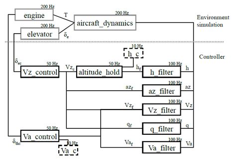
This exercise shows how to synchronize dataflows and control flows
in a simplified Flight Control System. The exercice is inspired from
the Claire Pageti RTAS 2014 article
(Pagetti 2014).
This figure is also extracted from
(Pagetti 2014).
We assume the following tasks parameters for this case study:
| Tasks | Execution times | Periods |
| Engine | 100 us | 5000 us |
| Aircraft_Dynamics | 200 us | 5000 us |
| Elevator | 100 us | 5000 us |
| Elevator | 100 us | 5000 us |
| H_Filter | 100 us | 10000 us |
| Vz_control | 100 us | 20000 us |
| Altitude_Hold | 100 us | 20000 us |
| Va_Filter | 100 us | 10000 us |
| Az_Filter | 100 us | 10000 us |
| Vz_Filter | 100 us | 10000 us |
| Q_Filter | 100 us | 10000 us |
| Va_control | 100 us | 20000 us |
| Monitoring | 100 us | 10000 us |
- Question 1:
- Download
this AADL model
which represents a possible AADL design for the functional
model shown above. Note the use of Feature Groups and Thread Groups.
- Identify what are the main missing AADL constructs to run scheduling analysis.
- To help you, you can use AADLInspector: load the model and try to run scheduling analysis.
- Question 2:
- Add missing connections in THREAD GROUP IMPLEMENTATION Flight_Software.impl
- Add missing data for scheduling analysis and run scheduling analysis.
- Question 3:
- Add Priority and/or Dispatch_Offset properties in order to ensure
a proper ordering of the threads regarding the dataflow logics.
- Again, check with the scheduling analysis tools.
Possible solution/AADL model for this
case study here.